说明 GPU 计算的三种方法：曼德布洛特集合

此示例展示如何调整您的 MATLAB® 代码以使用 GPU 计算曼德布洛特集合。

从现有算法开始，此示例展示了如何使用 Parallel Computing Toolbox™ 调整代码以通过三种方式利用 GPU 硬件：

使用现有算法，但以 GPU 数据作为输入
使用 arrayfun 对每个元素独立执行算法
使用 MATLAB/CUDA® 接口运行现有 CUDA/C++ 代码

设置

以下值指定了位于主心形线和其左侧 p/q 球状线之间的谷地中曼德布洛特集的高度缩放部分。

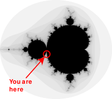
在这些限制之间创建一个 1000x1000 的实部 (X) 和虚部 (Y) 网格，并且在每个网格位置上迭代 Mandelbrot 算法 500 次。

maxIterations = 500;
gridSize = 1000;
xlim = [-0.748766713922161, -0.748766707771757];
ylim = [ 0.123640844894862,  0.123640851045266];

MATLAB 中的曼德布洛特集

下面是使用标准 MATLAB 命令在 CPU 上运行的曼德布洛特集的实现。这是基于 Cleve Moler 的 Experiments with MATLAB 电子书中提供的代码。使用 tic 和 toc 来计时 CPU 上的执行时间。

设置复值的二维网格。

tic;
x = linspace(xlim(1),xlim(2),gridSize);
y = linspace(ylim(1),ylim(2),gridSize);

[xGrid,yGrid] = meshgrid(x,y);
z0 = xGrid + 1i*yGrid;

对于 500 次迭代，通过对前一个值的平方并添加其初始值 z 来计算复杂网格 z0 上某个点的下一个值。计算 z 的幅度小于或等于二的迭代次数。该计算是向量化的，以便每个位置都立即更新。

cpuCount = ones(size(z0));
z = z0;
for n = 0:maxIterations
    z = z.*z + z0;
    inside = abs(z)<=2;
    cpuCount = cpuCount + inside;
end
cpuCount = log(cpuCount);
cpuTime = toc

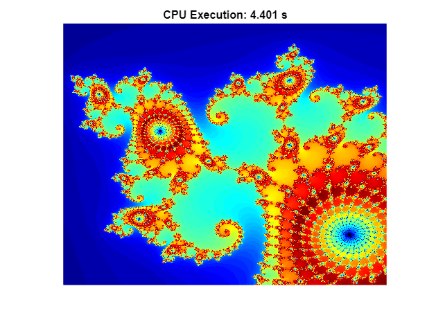
cpuTime = 4.4007

绘制计数的自然对数。

figure
imagesc(x,y,cpuCount);
c = colormap([jet;flipud(jet);0 0 0]);
axis off
title(sprintf("CPU Execution: %1.3f s",cpuTime));

使用 `gpuArray`

当 MATLAB 在 GPU 上遇到数据时，就会在 GPU 上执行使用该数据的计算。gpuArray 类提供了许多函数的 GPU 版本，您可以使用它们来创建数据数组，包括此处所需的 linspace、logspace 和 meshgrid 函数。类似地，使用函数ones 直接在 GPU 上初始化 count 数组。

确保您想要的 GPU 可用且已被选择。

gpu = gpuDevice;
disp(gpu.Name + " GPU selected.")

NVIDIA RTX A5000 GPU selected.

调用 naiveGPUMandelbrot 函数。支持函数 naiveGPUMandelbrot 将 Mandelbrot 算法应用于 GPU 上网格上的每个点，并在本示例的末尾提供。

[x,y,naiveGPUCount] = naiveGPUMandelbrot(xlim,ylim,gridSize,maxIterations);

使用 gputimeit 来计时 GPU 上该函数的执行情况。对于使用 GPU 的函数，gputimeit 比 tic 和 toc 或 timeit 更好，因为它可以确保在记录经过的时间之前完成 GPU 上的所有操作。

naiveGPUTime = gputimeit(@() naiveGPUMandelbrot(xlim,ylim,gridSize,maxIterations))

naiveGPUTime = 0.2181

元素级操作

注意到该算法对输入的每个元素都同等操作，我们可以将代码放在函数中并使用 arrayfun 调用它。函数 processMandelbrotElement 在本示例末尾作为支持函数提供。对于 gpuArray 输入，与 arrayfun 一起使用的函数会被编译成本机 GPU 代码。

由于函数 processMandelbrotElement 仅处理单个元素，因此该函数引入了早期中止。对于曼德布洛特集的大多数视图，相当数量的元素很早就停止了，这可以节省大量的处理。for 循环也被 while 循环取代，因为它们通常更高效。此函数未提及 GPU，也不使用任何 GPU 特定功能。

使用 arrayfun 会导致 MATLAB 对执行整个计算的并行 GPU 操作进行一次调用，而不是对单独的 GPU 优化操作进行数千次调用（每次迭代至少 6 次）。第一次调用 arrayfun 在 GPU 上运行特定函数时，需要一些额外时间来设置该函数以供 GPU 执行。后续使用相同函数调用 arrayfun 可以运行得更快。

设置复值的二维网格。

xGrid = gpuArray(xGrid);
yGrid = gpuArray(yGrid);

使用 arrayfun，对网格上的每个点应用 Mandelbrot 算法。

gpuArrayfunCount = arrayfun(@processMandelbrotElement, ...
                  xGrid,yGrid,maxIterations);

使用 arrayfun 来计时 gputimeit 的执行。

gpuArrayfunTime = gputimeit(@() arrayfun(@processMandelbrotElement, ...
                  xGrid,yGrid,maxIterations))

gpuArrayfunTime = 0.0308

使用 CUDA

在 MATLAB 中的试验中，通过将基本算法转换为 C-Mex 函数，性能得到了提高。如果您愿意进行一些 C/C++编程工作，那么您可以使用 Parallel Computing Toolbox™ 调用预先编写的 CUDA 内核，并使用 MATLAB 数据。有关在 MATLAB 中使用 CUDA 内核的更多详细信息，请参阅在 GPU 上运行 CUDA 或 PTX 代码。

本示例 pctdemo_processMandelbrotElement.cu 提供了元素处理算法的 CUDA/C++ 实现。下面给出了针对单个位置执行 Mandelbrot 算法的 CUDA/C++ 代码部分。

__device__
unsigned int doIterations( double const realPart0, 
                           double const imagPart0, 
                           unsigned int const maxIters ) {
   // Initialize: z = z0
   double realPart = realPart0;
   double imagPart = imagPart0;
   unsigned int count = 0;
   // Loop until escape
   while ( ( count <= maxIters )
          && ((realPart*realPart + imagPart*imagPart) <= 4.0) ) {
      ++count;
      // Update: z = z*z + z0;
      double const oldRealPart = realPart;
      realPart = realPart*realPart - imagPart*imagPart + realPart0;
      imagPart = 2.0*oldRealPart*imagPart + imagPart0;
   }
   return count;
}

使用 mexcuda 将此文件编译为并行线程执行 (PTX) 文件。

mexcuda -ptx pctdemo_processMandelbrotElement.cu

Building with 'NVIDIA CUDA Compiler'.
MEX completed successfully.

通过将 CUDA 文件和 PTX 文件传递给 parallel.gpu.CUDAKernel 函数来创建 parallel.gpu.CUDAKernel 对象。

cudaFilename = "pctdemo_processMandelbrotElement.cu";
ptxFilename = "pctdemo_processMandelbrotElement.ptx";
kernel = parallel.gpu.CUDAKernel(ptxFilename,cudaFilename);

曼德布洛特集合中每个位置都需要一个 GPU 线程，线程分组为块。内核指示线程块有多大。计算所需的线程块数量，并相应地设置内核的 GridSize 属性（实际上是 GPU 将独立启动的线程块数量）。

numElements = numel(xGrid);
kernel.ThreadBlockSize = [kernel.MaxThreadsPerBlock,1,1];
kernel.GridSize = [ceil(numElements/kernel.MaxThreadsPerBlock),1];

使用 feval 计算内核。

count = zeros(size(xGrid),"gpuArray");
gpuCUDAKernelCount = feval(kernel,count,xGrid,yGrid,maxIterations,numElements);

使用 gputimeit 来计时内核执行。

gpuCUDAKernelTime = gputimeit(@() feval(kernel,count,xGrid,yGrid,maxIterations,numElements));

摘要

绘制不同方法的结果并比较执行时间。

method = ["Naive GPU Execution" "GPU Execution Using arrayfun" "CUDAKernel Execution"];
count = cat(3,naiveGPUCount,gpuArrayfunCount,gpuCUDAKernelCount);
time = [naiveGPUTime gpuArrayfunTime gpuCUDAKernelTime];

figure
colormap(c)
tiledlayout("flow")
nexttile
imagesc(x,y,cpuCount);
axis off
title(sprintf("CPU Execution: %1.3f s",cpuTime));

for idx = 1:3
nexttile
imagesc(x,y,count(:,:,idx))
axis off
title(sprintf("%s: %1.3f s \n  (%1.1fx faster)", ...
    method(idx),time(idx),cpuTime/time(idx)))
end

此示例展示了调整 MATLAB 算法以利用 GPU 硬件的三种方法：

使用gpuArray将输入数据转换为 GPU 上的数据，保持算法不变。
在 gpuArray 输入上使用 arrayfun 对输入的每个元素独立执行算法。
使用 parallel.gpu.CUDAKernel 使用 MATLAB 数据运行一些现有的 CUDA/C++ 代码。

本示例中的代码在配备 NVIDIA® RTX A5000 GPU 的 Windows® 10、Intel® Xeon® W-2133 @ 3.60 GHz 测试系统上计时。

支持函数

支持函数 naiveGPUMandelbrot 创建了一个二维复值网格，并计算复值数 (x0,y0) 跳出复平面上半径为 2 的圆之前的迭代次数。每次迭代涉及映射 z = z^2 + z0 和 z0 = x0 + i*y0。该函数返回网格坐标向量和逃逸处的迭代计数的对数，如果点没有逃逸，则返回 maxIterations。通过在 GPU 上初始化数据并对该数据进行操作，naiveGPUMandelbrot 函数在 GPU 上执行 Mandelbrot 算法。

function [x,y,count] = naiveGPUMandelbrot(xlim,ylim,gridSize,maxIterations)

x = gpuArray.linspace(xlim(1),xlim(2),gridSize);
y = gpuArray.linspace(ylim(1),ylim(2),gridSize);
[xGrid,yGrid] = meshgrid(x,y);

z0 = complex(xGrid,yGrid);
count = ones(size(z0),"gpuArray");
z = z0;

for n = 0:maxIterations
    z = z.*z + z0;
    inside = abs(z)<=2;
    count = count + inside;
end

count = log(count);

end

支持函数 processMandelbrotElement 创建了一个二维复值网格，并计算复值数 (x0,y0) 跳出复平面上半径为 2 的圆之前的迭代次数。每次迭代涉及映射 z = z^2 + z0 和 z0 = x0 + i*y0。如果点未逃逸，则该函数返回逃逸时的迭代计数的对数或 maxIterations。

function count = processMandelbrotElement(x0,y0,maxIterations)

z0 = complex(x0,y0);
z = z0;
count = 1;

while (count <= maxIterations) && (abs(z) <= 2)
    count = count + 1;
    z = z*z + z0;
end

count = log(count);

end

另请参阅

gpuArray | arrayfun