Main Content

applyBoundaryCondition

Add boundary condition to PDEModel container

Description

applyBoundaryCondition(model,"dirichlet",RegionType,RegionID,Name,Value) adds a Dirichlet boundary condition to model. The boundary condition applies to boundary regions of type RegionType with ID numbers in RegionID, and with arguments r, h, u, EquationIndex specified in the Name,Value pairs. For Dirichlet boundary conditions, specify either both arguments r and h, or the argument u. When specifying u, you can also use EquationIndex.

example

applyBoundaryCondition(model,"neumann",RegionType,RegionID,Name,Value) adds a Neumann boundary condition to model. The boundary condition applies to boundary regions of type RegionType with ID numbers in RegionID, and with values g and q specified in the Name,Value pairs.

example

applyBoundaryCondition(model,"mixed",RegionType,RegionID,Name,Value) adds an individual boundary condition for each equation in a system of PDEs. The boundary condition applies to boundary regions of type RegionType with ID numbers in RegionID, and with values specified in the Name,Value pairs. For mixed boundary conditions, you can use Name,Value pairs from both Dirichlet and Neumann boundary conditions as needed.

example

bc = applyBoundaryCondition(___) returns the boundary condition object.

Examples

collapse all

Create a PDE model and geometry.

model = createpde(1);
R1 = [3,4,-1,1,1,-1,-.4,-.4,.4,.4]';
g = decsg(R1);
geometryFromEdges(model,g);

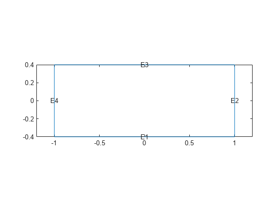
View the edge labels.

pdegplot(model,"EdgeLabels","on")
xlim([-1.2,1.2])
axis equal

Figure contains an axes object. The axes object contains 5 objects of type line, text.

Apply zero Dirichlet condition on the edge 1.

applyBoundaryCondition(model,"dirichlet", ...
                             "Edge",1,"u",0);

On other edges, apply Dirichlet condition h*u = r, where h = 1 and r = 1.

applyBoundaryCondition(model,"dirichlet", ...
                             "Edge",2:4, ...
                             "r",1,"h",1);

Create a PDE model and geometry.

model = createpde(2);
R1 = [3,4,-1,1,1,-1,-.4,-.4,.4,.4]';
g = decsg(R1);
geometryFromEdges(model,g);

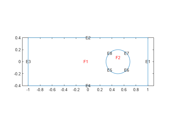
View the edge labels.

pdegplot(model,"EdgeLabels","on")
xlim([-1.2,1.2])
axis equal

Figure contains an axes object. The axes object contains 5 objects of type line, text.

Apply the following Neumann boundary conditions on the edge 4.

applyBoundaryCondition(model,"neumann", ...
                             "Edge",4, ...
                             "g",[0;.123], ...
                             "q",[0;0;0;0]);

Apply both types of boundary conditions to a scalar problem. First, create a PDE model and import a simple block geometry.

model = createpde;
importGeometry(model,"Block.stl");

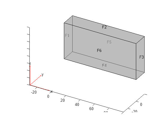
View the face labels.

pdegplot(model,"FaceLabels","on","FaceAlpha",0.5)

Figure contains an axes object. The axes object contains 6 objects of type quiver, text, patch, line.

Set zero Dirichlet conditions on the narrow faces, which are labeled 1 through 4.

applyBoundaryCondition(model,"dirichlet", ...
                             "Face",1:4,"u",0);

Set Neumann boundary conditions with opposite signs on faces 5 and 6.

applyBoundaryCondition(model,"neumann", ...
                             "Face",5,"g",1);
applyBoundaryCondition(model,"neumann", ...
                             "Face",6,"g",-1);

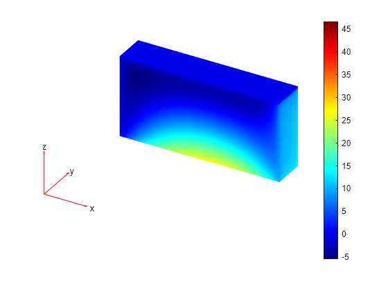
Solve an elliptic PDE with these boundary conditions, and plot the result.

specifyCoefficients(model,"m",0,"d",0,"c",1,"a",0,"f",0);
generateMesh(model);
results = solvepde(model);
u = results.NodalSolution;
pdeplot3D(model,"ColorMapData",u)

Figure contains an axes object. The hidden axes object contains 5 objects of type patch, quiver, text.

Create a PDE model and import a simple block geometry.

model = createpde(3);
importGeometry(model,"Block.stl");

View the face labels.

pdegplot(model,"FaceLabels","on","FaceAlpha",0.5)

Figure contains an axes object. The axes object contains 6 objects of type quiver, text, patch, line.

Set zero Dirichlet conditions on faces 1 and 2.

applyBoundaryCondition(model,"dirichlet", ...
                             "Face",1:2,"u",[0,0,0]);

Set Neumann boundary conditions with opposite signs on faces 4, 5, and 6.

applyBoundaryCondition(model,"neumann", ...
                             "Face",4:5,"g",[1;1;1]);
applyBoundaryCondition(model,"neumann", ...
                             "Face",6,"g",[-1;-1;-1]);

For face 3, apply generalized Neumann boundary condition for the first equation and Dirichlet boundary conditions for the second and third equations.

h = [0 0 0;0 1 0;0 0 1];
r = [0;3;3];
q = [1 0 0;0 0 0;0 0 0];
g = [10;0;0];
applyBoundaryCondition(model,"mixed","Face",3, ...
                       "h",h,"r",r,"g",g,"q",q);

Solve an elliptic PDE with these boundary conditions, and plot the result.

specifyCoefficients(model,"m",0,"d",0,"c",1, ...
                          "a",0,"f",[0;0;0]);
generateMesh(model);
results = solvepde(model);
u = results.NodalSolution;
pdeplot3D(model,"ColorMapData",u(:,1))

Figure contains an axes object. The hidden axes object contains 5 objects of type patch, quiver, text.

Input Arguments

collapse all

PDE model, specified as a PDEModel object.

Example: model = createpde

Geometric region type, specified as "Face" for 3-D geometry or "Edge" for 2-D geometry.

Example: applyBoundaryCondition(model,"dirichlet","Face",3,"u",0)

Data Types: char | string

Geometric region ID, specified as a vector of positive integers. Find the region IDs using pdegplot with the "FaceLabels" (3-D) or "EdgeLabels" (2-D) value set to "on".

Example: applyBoundaryCondition(model,"dirichlet","Face",3:6,"u",0)

Data Types: double

Name-Value Arguments

Example: applyBoundaryCondition(model,"dirichlet","Face",1:4,"u",0)

Dirichlet condition h*u = r, specified as a vector with N elements or a function handle. N is the number of PDEs in the system. For the syntax of the function handle form of r, see Nonconstant Boundary Conditions.

Example: "r",[0;4;-1]

Data Types: double | function_handle
Complex Number Support: Yes

Dirichlet condition h*u = r, specified as an N-by-N matrix, a vector with N^2 elements, or a function handle. N is the number of PDEs in the system. For the syntax of the function handle form of h, see Nonconstant Boundary Conditions.

Example: "h",[2,1;1,2]

Data Types: double | function_handle
Complex Number Support: Yes

Generalized Neumann condition n·(c×u) + qu = g, specified as a vector with N elements or a function handle. N is the number of PDEs in the system. For scalar PDEs, the generalized Neumann condition is n·(cu) + qu = g. For the syntax of the function handle form of g, see Nonconstant Boundary Conditions.

Example: "g",[3;2;-1]

Data Types: double | function_handle
Complex Number Support: Yes

Generalized Neumann condition n·(c×u) + qu = g, specified as an N-by-N matrix, a vector with N^2 elements, or a function handle. N is the number of PDEs in the system. For the syntax of the function handle form of q, see Nonconstant Boundary Conditions.

Example: "q",eye(3)

Data Types: double | function_handle
Complex Number Support: Yes

Dirichlet conditions, specified as a vector of up to N elements or as a function handle. If u has less than N elements, then you must also use EquationIndex. The u and EquationIndex arguments must have the same length. If u has N elements, then specifying EquationIndex is optional.

For the syntax of the function handle form of u, see Nonconstant Boundary Conditions.

Example: applyBoundaryCondition(model,"dirichlet","Face",[2,4,11],"u",0)

Data Types: double
Complex Number Support: Yes

Index of the known u components, specified as a vector of integers with entries from 1 to N. EquationIndex and u must have the same length.

When using EquationIndex to specify Dirichlet boundary conditions for a subset of components, use the mixed argument instead of dirichlet. The remaining components satisfy the default Neumann boundary condition with the zero values for "g" and "q".

Example: applyBoundaryCondition(model,"mixed","Face",[2,4,11],"u",[3,-1],"EquationIndex",[2,3])

Data Types: double

Vectorized function evaluation, specified as "on" or "off". This evaluation applies when you pass a function handle as an argument. To save time in function handle evaluation, specify "on", assuming that your function handle computes in a vectorized fashion. See Vectorization. For details of this evaluation, see Nonconstant Boundary Conditions.

Example: applyBoundaryCondition(model,"dirichlet","Face",[2,4,11],"u",@ucalculator,"Vectorized","on")

Data Types: char | string

Output Arguments

collapse all

Boundary condition, returned as a BoundaryCondition Properties object. The model object contains a vector of BoundaryCondition objects. bc is the last element of this vector.

Tips

  • When there are multiple boundary condition assignments to the same geometric region, the toolbox uses the last applied setting.

  • To avoid assigning boundary conditions to a wrong region, ensure that you are using the correct geometric region IDs by plotting and visually inspecting the geometry.

  • If you do not specify a boundary condition for an edge or face, the default is the Neumann boundary condition with the zero values for "g" and "q".

Version History

Introduced in R2015a