Custom DQN Training Loop with LSTM Network

This example uses:

This example shows how to use a custom training loop to train a deep Q-learning network (DQN) agent with a Long Short-Term Memory (LSTM) network. Specifically, in this example, you train the agent to control a house heating system modeled in Simscape™. For an example in which you train a default DQN agent with an LSTM network to control a house heating system, Train DQN Agent with LSTM Network to Control House Heating System. For more information on the DQN training algorithm, see Deep Q-Network (DQN) Agent.

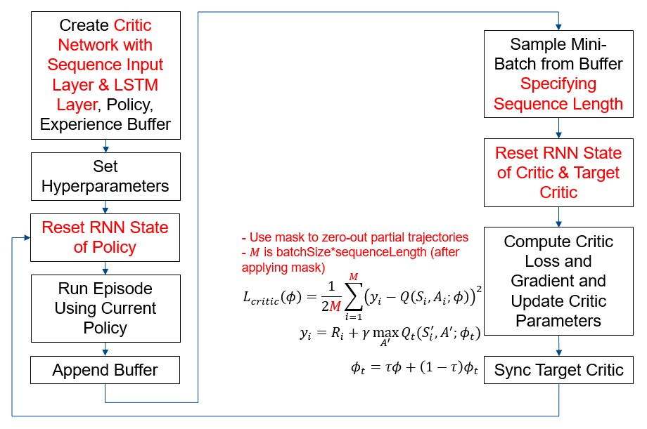
The figure below summarizes the workflow for training the agent. The red text highlights steps that are specific to LSTM networks.

Preserve Random Number Sequence for Reproducibility

Some sections in this example require random number computations. Specify the seed and random number generator algorithm at the beginning of a section to use the same random number sequence each time you run it. Preserving the random number sequence allows you to reproduce the results of the section. For more information, see Results Reproducibility.

Set the random number seed to 0 and the algorithm to Mersenne Twister. For more information, see rng.

previousRngState = rng(0,"twister");

The output previousRngState is a structure that contains information about the previous state of the sequence. You will restore the state at the end of the example.

House Heating Simulink Model

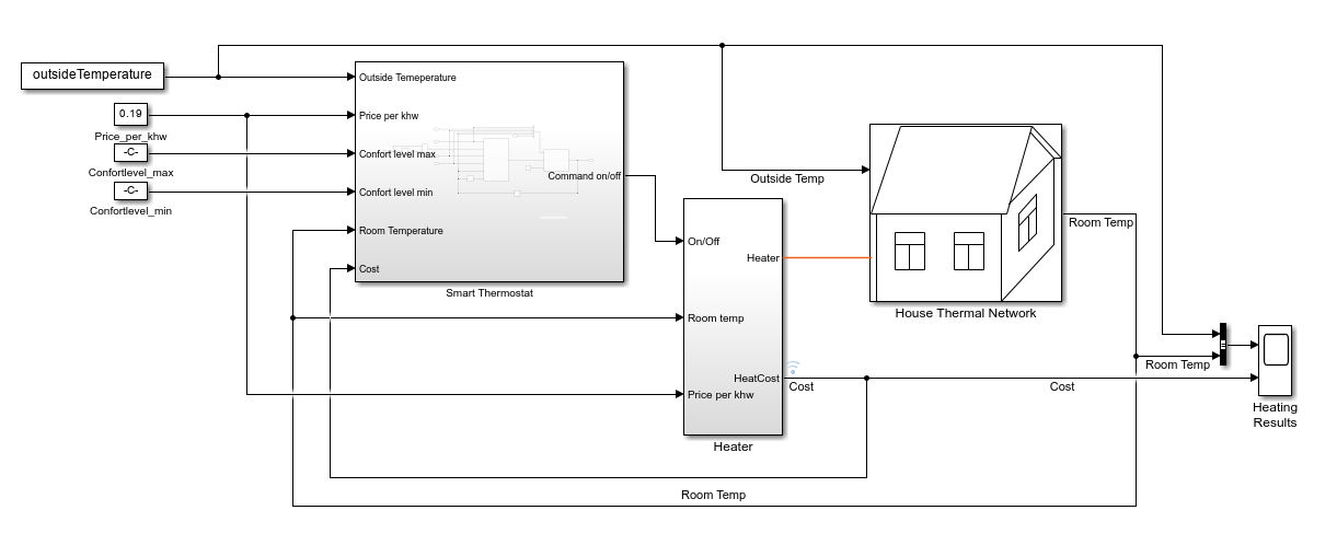
The reinforcement learning (RL) environment for this example uses the Simulink® model described in the House Heating System (Simscape) example.The model contains a heater block, a thermostat block (which contains an RL agent block and a reward block) and the House Thermal Network block (modeled in Simscape). Heat moves between the interior of the home and the outside environment through the walls, windows, and roof. You use weather station data between March 21 and April 15, 2022, to simulate the outside temperature. For more information about the data acquisition, see Compare Temperature Data from Three Different Days (ThingSpeak).

The training goal for the custom training loop is to minimize the energy cost and maximize the amount of time the house is in the comfortable temperature range by turning on/off the heater. The house is comfortable when its interior temperature $T_{room}$ is between $T_{comfortMin}$ and $T_{comfortMax}$ .

The reinforcement learning problem is defined as follows:

The observation is a 6-dimensional column vector that consists of the room temperature ( $^{\circ} C$ ), outside temperature ( $^{\circ} C$ ), maximum comfort temperature ( $^{\circ} C$ ), minimum comfort temperature ( $^{\circ} C$ ), last action, and price per kWh (USD).
The action is discrete. Specifically, the action 0 represents turning the heater off, and the action 1 represents turning it on.
The reward block calculates the total reward $R$ as the sum of the comfort reward $Rc$ and a penalty for switching $Ps$ , from which an energy cost $Ce$ is subtracted: $R = Rc + Ps - Ce$ . These three components are defined as follows.

$Rc = {\begin{array}{ll} 0.1 & if {T_{comfortMin} \leq T}_{room} \leq T_{comfortMax} \\ - w | T_{room} - T_{comfortMin} | & if T_{room} < T_{comfortMin} \\ - w | T_{room} - T_{comfortMax} | & if T_{room} > T_{comfortMax} \end{array}$

where $w = 0.1$ , $T_{comfortMin} = 18,$ and $T_{comfortMax} = 23$ .

$Ps = {\begin{array}{ll} - 0.01 & if a_{t} \neq a_{t - 1} where a_{t} is the current action and a_{t - 1} is the previous action \\ 0 & otherwise \end{array}$

$Ce = CostPerStep = PricePerKwh * ElectricityUsed$

The reward function is inspired by [1].

The Is-Done signal supplied to the RL Agent block is always 0, indicating that there is no early termination condition.

Define Simulink Environment

Open the model.

mdl = "rlHouseHeatingSystemDQNLSTMCustomLoop";
open_system(mdl)

Define the sample time and the maximum number of steps per episode. You need these variables for the script and reset functions.

sampleTime = 120; % seconds
maxStepsPerEpisode = 1000;

Assign the agent block path information to the agentBlk variable, for later use.

agentBlk = mdl + "/Smart Thermostat/RL Agent";

Load the outside temperature data to simulate the environment temperature.

data = load('temperatureMar21toApr15_2022CustomLoop.mat');
temperatureData = data.temperatureData;

Extract validation data.

temperatureMarch21 = temperatureData(1:60*24,:);
temperatureApril15 = temperatureData(end-60*24+1:end,:);

Extract training data.

temperatureData = temperatureData(60*24+1:end-60*24,:);

The Simulink model loads the outside temperature history, the maximum comfort temperature, and the minimum comfort temperature. These variables are part of the observation vector.

outsideTemperature = temperatureData;
comfortMax = 23;
comfortMin = 18;

Define the observation and action specifications.

obsInfo = rlNumericSpec([6,1]);
actInfo = rlFiniteSetSpec([0,1]); % (0=off,1=on)

Create an environment object for the house heating environment.

env = rlSimulinkEnv(mdl,agentBlk,obsInfo,actInfo);

Specify a custom reset function. Use hRLHeatingSystemCustomLoopResetFcn to reset the environment at the beginning of each episode. This function randomly selects a time between March 22 and April 14 such that at least maxStepsPerEpisode samples are available. The environment uses this time as the initial time for the outside temperatures. For more information, see Reset Function for Simulink Environments.

env.ResetFcn = @(in) hRLHeatingSystemCustomLoopResetFcn(in,...
    temperatureData,maxStepsPerEpisode,sampleTime);

Create Critic, Policy, and Experience Buffer

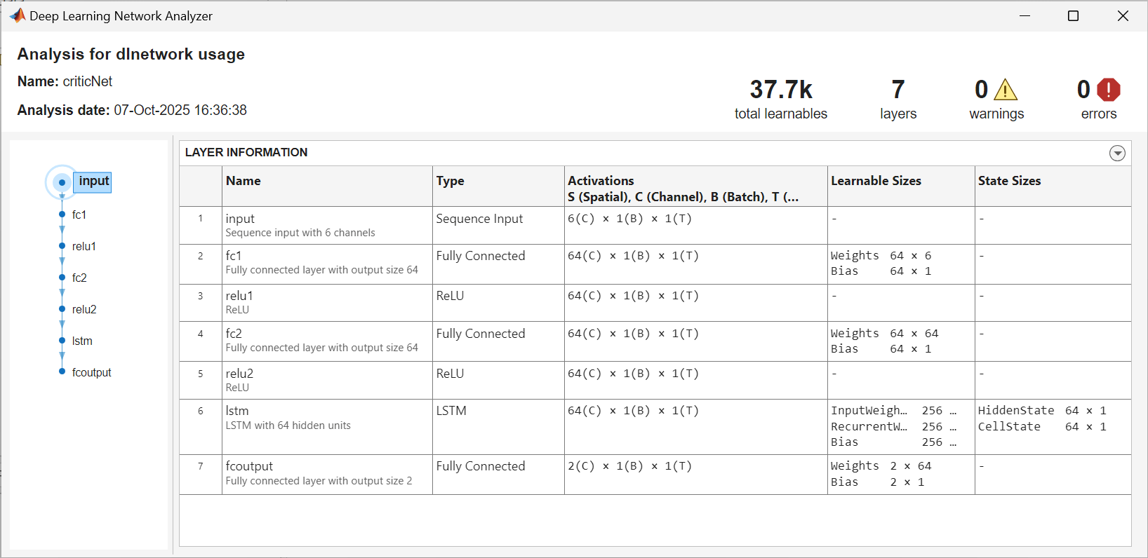
Create a critic network. The createCriticNet function is defined at the end of this example. Note that a sequenceInputLayer is used in conjunction with LSTM layers to represent a RNN (recurrent neural network). For more information, see sequenceInputLayer.

criticNet = createCriticNet(obsInfo,actInfo);
analyzeNetwork(criticNet);

Create a critic and target critic. For more information, see rlVectorQValueFunction.

agentData.Critic = rlVectorQValueFunction(criticNet,obsInfo,actInfo);
agentData.TargetCritic = agentData.Critic;

To speed up the gradient computation, use dlaccelerate to accelerate the loss function. The criticLossFcn function is defined at the end of this example.

agentData.AccelCriticGrad = dlaccelerate(@criticLossFcn);

Create an epsilon-greedy policy object. For more information, see rlEpsilonGreedyPolicy.

policy = rlEpsilonGreedyPolicy(agentData.Critic);
policy.UseEpsilonGreedyAction = true;
policy.SampleTime = sampleTime;
policy.ExplorationOptions.Epsilon = 1;
policy.ExplorationOptions.EpsilonDecay = 1e-4;
policy.ExplorationOptions.EpsilonMin = 0.01;

Use rlOptimizer to create optimizer objects for updating the critic.

Set the learning rate to 1e-3.
Set the gradient threshold to 1 to avoid large gradients.

optimizerOpt = rlOptimizerOptions(LearnRate=1e-3, GradientThreshold=1);
agentData.CriticOptimizer = rlOptimizer(optimizerOpt);

Create Experience Buffer

Create an experience buffer for the agent with a maximum length of 1e6. For more information, see rlReplayMemory.

replayMemorySize = 1e6;
agentData.Replay = rlReplayMemory(obsInfo,actInfo,replayMemorySize);

When using a recurrent neural network, you must set SequenceLength to a value greater than 1. This value is used in training to determine the length of the minibatch used to calculate the gradient. For more information about LSTM layers, see Long Short-Term Memory Neural Networks.

For this example, set SequenceLength to 20.

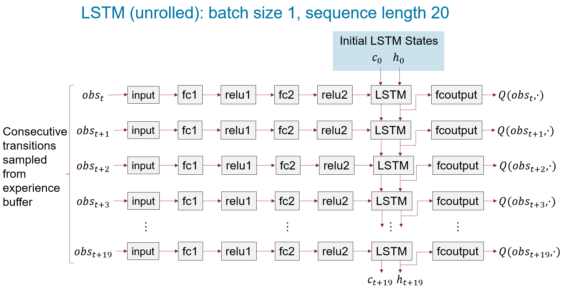
agentData.SequenceLength = 20;

The figure below shows an LSTM network unrolled for batch size of 1 and sequence length of 20.

Create a structure to store additional data required for training the critic.

agentData.MaxEpisodes = 500;
agentData.DiscountFactor = 0.99;
agentData.MiniBatchSize = 64;
agentData.MaxMiniBatchPerEpoch = 100;
agentData.NumEpochs = 1;
agentData.TargetSmoothFactor = 1e-3;

Set Up Training and Create Data Logger

Create a file data logger object using the rlDataLogger function. Open the Reinforcement Learning Data Viewer tool to visualize the logged data during training. For more information, see rlDataLogger and rlDataViewer.

To save time while running this example, load a pretrained agent by setting doTraining to false. To train the agent yourself, set doTraining to true.

doTraining = false;
useLogger = false;
if useLogger && doTraining
    logger = rlDataLogger();
    rlDataViewer(logger);
    setup(logger);
end

agentData.StopTrainingValue = 85;
agentData.AverageReward = 0;
agentData.ScoreAveragingWindowLength = 5;

Run Training Loop

To reproduce the results of this section, set random seed and algorithm.

rng(0,"twister");

Execute the custom training loop. In this example:

The runEpisode function simulates the agent in the environment for one episode.
To speed up training, set the CleanupPostSim option to false when calling runEpisode. This setting keeps the model compiled between episodes.
Once the experience buffer contains at least agentData.MiniBatchSize samples, the algorithm updates the agent at the end of each episode using the updateAgent function defined at the end of this example.
After all of the episodes are complete, the cleanup function cleans up the environment.

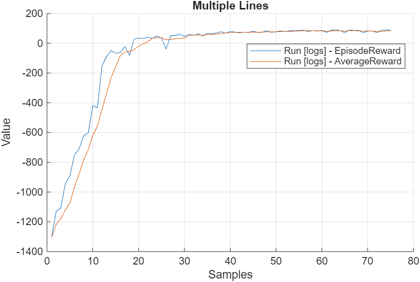
% Create variable to store the cumulative rewards of all episodes.
rewardAllEpisodes = zeros(agentData.MaxEpisodes,1);

% Evaluate the agent every 25 training episodes.
evaluatorFrequency = 25;  

if doTraining
    for episodeIdx = 1:agentData.MaxEpisodes
    
        agentData.EpisodeIdx = episodeIdx;
        
        % Reset RNN state of policy to zeros.
        policy.QValueFunction.State = ...
            cellfun(@(x) zeros(size(x), 'like', x), ...
            policy.QValueFunction.State, 'UniformOutput', false);

        % Run an episode to simulate the environment with the policy.
        out = runEpisode(env,policy,...
            MaxSteps=maxStepsPerEpisode,CleanupPostSim=false);
    
        % Append experience to replay memory buffer.
        append(agentData.Replay,out.AgentData.Experiences);
        
        % Extract episode information to update the training curves.
        episodeInfo = out.AgentData.EpisodeInfo;
    
        % Extract the policy for the next episode.
        policy = out.AgentData.Agent;
    
        % Extract the cumulative reward.
        cumulativeRwd = episodeInfo.CumulativeReward;
        rewardAllEpisodes(episodeIdx) = cumulativeRwd;
        
        if agentData.Replay.Length>=agentData.MiniBatchSize
            % Learn when the agent has collected enough data.
            % The updateAgent function updates the critic 
            % and the target critic networks.
            agentData = updateAgent(agentData);

            % Update the policy parameters using the critic parameters.
            policy = setLearnableParameters( ...
                policy,getLearnableParameters(agentData.Critic));
        end
    
        % Compute average reward.
        if episodeIdx>agentData.ScoreAveragingWindowLength
            averageReward = mean(rewardAllEpisodes(episodeIdx-...
                agentData.ScoreAveragingWindowLength+1:episodeIdx));
        else
            averageReward = mean(rewardAllEpisodes(1:episodeIdx));
        end
        
        % Log data.
        if useLogger
            store(logger, "EpisodeReward", cumulativeRwd, episodeIdx);
            store(logger, "AverageReward", averageReward, episodeIdx);
            drawnow();
            write(logger);
        end
        
        % Evaluate the policy every evaluatorFrequency episodes.
        if mod(episodeIdx,evaluatorFrequency)==0
            % Reset RNN state of policy to zeros.
            policy.QValueFunction.State = cellfun( ...
                @(x) zeros(size(x), 'like', x), ...
                policy.QValueFunction.State, 'UniformOutput', false);

            % Evaluate the trained policy by turning off exploration.
            policy.UseEpsilonGreedyAction = 0;
            numSimulations = 3;
            simOptions = rlSimulationOptions("MaxSteps",...
                maxStepsPerEpisode,"NumSimulations",numSimulations);
            simOut = sim(env,policy,simOptions);
            simCumReward = zeros(numSimulations,1);
            for ii=1:numSimulations
                simCumReward(ii) = sum(simOut(ii).Reward);
            end
            
            % Exit the training loop if the cumulative reward exceeds 
            % StopTrainingValue.
            if mean(simCumReward)>=agentData.StopTrainingValue
                break;
            end

            % Turn on exploration for the next episode.
            policy.UseEpsilonGreedyAction = 1;
        end
        
        % Log the evaluation statistics.
        if useLogger
            if mod(episodeIdx,evaluatorFrequency)==0
                store(logger,"EvaluationStatistic", ...
                    mean(simCumReward),episodeIdx);
            else
                store(logger,"EvaluationStatistic",NaN,episodeIdx);
            end
        end

    end
    
    % Clean up the environment.
    cleanup(env);

    % Save the trained critic.
    trainedCritic = agentData.Critic;
    save("trainedAgentLSTMCustomLoop.mat","trainedCritic");
else
    % If you choose to skip the training loop, 
    % load the trained critic.
    load('trainedAgentLSTMCustomLoop.mat');
    
    % Create epsilon-greedy policy from the trained critic
    % for simulation.
    policy = rlEpsilonGreedyPolicy(trainedCritic);
    policy.UseEpsilonGreedyAction = 0;
    policy.SampleTime = sampleTime;
end

% cleanup
if useLogger && doTraining
    cleanup(logger);
end

The plot shows the reward obtained by the agent for each episode and the average reward over agentData.ScoreAveragingWindowLength.

Simulate the Trained Policy

To validate the performance of the trained policy, simulate it within the house heating environment. For more information on agent simulation, see rlSimulationOptions and sim.

To reproduce the results of this section, set random seed and algorithm.

rng(0, "twister");

Evaluate the performance of the trained policy using the validation temperature data from March 21, 2022, which was not used for training. To supply this data set, use the environment reset function hRLHeatingSystemValidateCustomLoopResetFcn.

maxSteps= 720;
validationTemperature = temperatureMarch21;
env.ResetFcn = @(in) hRLHeatingSystemValidateCustomLoopResetFcn( ...
    in,validationTemperature);
simOptions = rlSimulationOptions(MaxSteps = maxSteps);
experience1 = sim(env,policy,simOptions);

Use the plotResults function, provided at the end of the example, to visualize the performance of the trained policy.

plotResults(experience1, maxSteps, ...
    comfortMax, comfortMin, sampleTime,1);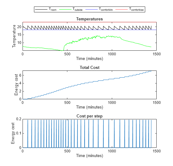

$Figure contains 3 axes objects. Axes object 1 with title Temperatures, xlabel Time (minutes), ylabel Temperature contains 4 objects of type line, constantline. These objects represent T_{room}, T_{outside}, T_{comfortMin}, T_{comfortMax}. Axes object 2 with title Total Cost, xlabel Time (minutes), ylabel Energy cost contains an object of type line. Axes object 3 with title Cost per step, xlabel Time (minutes), ylabel Energy cost contains an object of type line.$

Comfort Temperature violation: 0/1440 minutes, cost: 7.214489 dollars

Next, evaluate the trained policy's performance using the validation temperature data from April 15th, 2022.

% Validate trained policy using the data from April 15.
validationTemperature = temperatureApril15;
env.ResetFcn = @(in) hRLHeatingSystemValidateCustomLoopResetFcn( ...
    in,validationTemperature);
experience2 = sim(env,policy,simOptions);
plotResults( ...
    experience2, ...
    maxSteps, ...
    comfortMax, ...
    comfortMin, ...
    sampleTime,2)

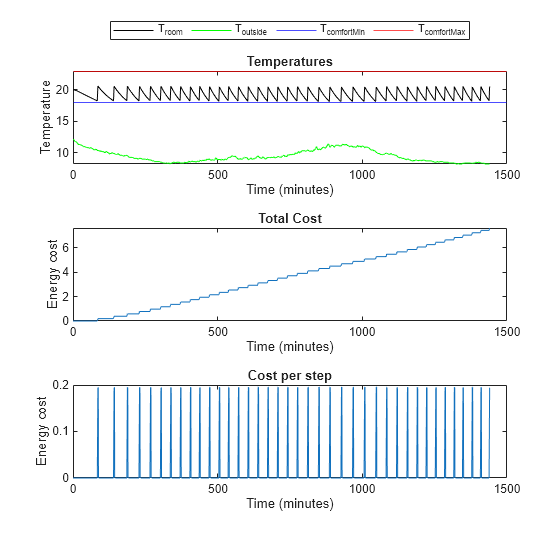
Comfort Temperature violation: 0/1440 minutes, cost: 7.604639 dollars

Evaluate the trained policy's performance when the temperature is mild. Add eight degrees to the temperatures from April 15th to create data for mild temperatures.

% Validate trained policy using the data from April 15 + 8 degrees.
validationTemperature = temperatureApril15;
validationTemperature(:,2) = validationTemperature(:,2) + 8;
env.ResetFcn = @(in) hRLHeatingSystemValidateCustomLoopResetFcn( ...
    in,validationTemperature);
experience3 = sim(env,policy,simOptions);
plotResults(experience3, ...
    maxSteps, ...
    comfortMax, ...
    comfortMin, ...
    sampleTime, ...
    3)

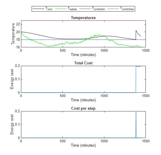
Comfort Temperature violation: 0/1440 minutes, cost: 0.195710 dollars

The trained policy performs well in all three scenarios.

Restore the random number stream using the information stored in previousRngState.

rng(previousRngState);

Local Functions

Create Critic Network

The createCriticNet function creates a custom network for the critic. Note that you must use a sequenceInputLayer in conjunction with LSTM layers to represent a RNN (recurrent neural network). For more information, see sequenceInputLayer.

function net = createCriticNet(obsInfo,actInfo)
    
    numObs = obsInfo.Dimension(1);
    numAct = getNumberOfElements(actInfo);

    net = [
        sequenceInputLayer(numObs)
        fullyConnectedLayer(64)
        reluLayer
        fullyConnectedLayer(64)
        reluLayer
        lstmLayer(64)
        fullyConnectedLayer(numAct)];
    
    net = dlnetwork(net);

end

Critic Loss

The criticLossFcn function computes the loss and the gradient to update the critic. Here, to compute loss only on the actual experiences, not the padding data, multiply the loss by the sequence padding mask that the updateAgent function calculates when it samples from the experience buffer. For more information, see rlReplayMemory and sample.

function [criticGradient, loss_data] = criticLossFcn( ...
    critic,observation,action_index,targetq,mask)
    
    % Obtain the number of non-padded experiences.
    N = sum(mask,"all");

    % Extract the action values, Q(s,a), corresponding to the current 
    % batch of observations.
    [q,~] = getValue(critic,observation,UseForward=true);
    % Choosing the q values corresponding to the actions taken.
    q = q(action_index);
    q = q';
    
    % Calculate the TD error.
    targetq = reshape(targetq,size(q));
    tdError = q-targetq;

    % Multiply loss by the sequence padding mask returned 
    % when sampling from the experience buffer to ignore 
    % padding. Compute the loss only over actual experiences.  
    tdError = tdError.*reshape(mask,size(tdError));
    % Loss is the half mean-square error of 
    % q = Q(observation,action) against targetq.
    criticLossValue = 0.5.*sum(tdError.^2,"all")/N;
    
    % Compute the gradient of the loss with respect to the critic
    % parameters.
    criticGradient = dlgradient(criticLossValue,critic.Learnables);
    
    loss_data.CriticLoss= criticLossValue;

end

Agent Update Function

The updateAgent function updates the critic and the target critic.To make sure that for each batch element the sampler draws up to SequenceLength consecutive transitions from the experience buffer, set the SequenceLength name-value argument of the sample function. To keep all batch elements at the same SequenceLength, shorter sampled sequences are padded and a logical mask marks real steps (true) vs padded steps (false) is returned. The criticLossFcn computes the loss only over real experiences by using this mask. For more information, see rlReplayMemory and sample.

function agentData = updateAgent(agentData)
    
    % Obtain the number of batches needed.
    numBatches = min( ...
        floor(agentData.Replay.Length/agentData.MiniBatchSize), ...
        agentData.MaxMiniBatchPerEpoch);

    for epoch = 1:agentData.NumEpochs
        % Get the batch data. 
        % To keep all batch elements at the same SequenceLength, 
        % shorter sampled sequences are padded and a logical mask 
        % marks real steps (true) vs padded steps (false)
        % is returned. The criticLossFcn use this mask to compute 
        % the loss only over real experiences.
        [superMiniBatch, superMiniBatchMask] = sample(agentData.Replay, ...
            numBatches*agentData.MiniBatchSize,...
            SequenceLength=agentData.SequenceLength,ReturnDlarray=true);

        % Shuffle batch indices every epoch.
        idxshuffled  = randperm(numBatches*agentData.MiniBatchSize);
        idxbeg = 1;
        idxend = idxbeg+agentData.MiniBatchSize-1;
        for iteration = 1:numBatches
            mbIdx = idxshuffled(idxbeg:idxend);
            idxbeg = idxend+1;
            idxend = idxbeg+agentData.MiniBatchSize-1;

            % Get the mini-batch data.
            mbObs = {superMiniBatch.Observation{:}(:,:,mbIdx,:)};
            mbNobs = {superMiniBatch.NextObservation{:}(:,:,mbIdx,:)};
            mbAct = {superMiniBatch.Action{:}(:,:,mbIdx,:)};
            mbReward = superMiniBatch.Reward(:,mbIdx,:);
            mbIsDone = superMiniBatch.IsDone(:,mbIdx,:);
            mbMask = superMiniBatchMask(:,mbIdx,:);
            
            % Reset RNN state of critic and target critic to zeros.
            agentData.Critic.State = cellfun( ...
                @(x) zeros(size(x), 'like', x), ...
                agentData.Critic.State, 'UniformOutput', false);
            agentData.TargetCritic.State = cellfun( ...
                @(x) zeros(size(x), 'like', x), ...
                agentData.TargetCritic.State, 'UniformOutput', false);

            % Compute target.
            mbY = mbReward + (mbIsDone~=1).*getMaxQValue( ...
                agentData.TargetCritic,mbNobs).*agentData.DiscountFactor;
            
            % Build a one-hot logical matrix of size 
            % (numElements, miniBatchSize*sequenceLength)
            % indicating, for each action element in ActionInfo, 
            % which batch entries select that action. 
            % Convert to dlarray.
            actionIndex = dlarray(localGetElementIndicationMatrix( ...
                agentData.Critic.ActionInfo, mbAct, numel(mbY)));
            
            % Compute critic gradient using the accelerated 
            % criticLossFcn function.
            [criticGradient, lossData] = dlfeval(agentData.AccelCriticGrad,...
                agentData.Critic,mbObs,actionIndex,mbY,mbMask);
            
            % Update the critic parameters.
            % For more information, see <docid:rl_ref#mw_f48d6602-fa23-4aa6-b26b-4ef23f8a405c update>.
            [agentData.Critic,agentData.CriticOptimizer] = update(...
                agentData.CriticOptimizer,agentData.Critic,...
                criticGradient);
            
            % Update targets using the TargetSmoothFactor hyper-parameter.
            agentData.TargetCritic = syncParameters( ...
                agentData.TargetCritic,...
                agentData.Critic, ...
                agentData.TargetSmoothFactor);

        end
    end

end

Get Element Indication Matrix

The localGetElementIndicationMatrix function returns a logical one-hot matrix with size (numElement,batchSize). For each action element defined in actInfo, the matrix indicates which batch entries select that action.

function elementMat = localGetElementIndicationMatrix( ...
    actInfo,batchElement,batchSize)
    % This function returns a True/False matrix 
    % with size (numElement,batchSize)

    num = getNumberOfElements(actInfo); % number of elements

    % Initialize element indication matrix.
    elementMat = false(num,batchSize);
    
    elementValuesFromSpec = actInfo.Elements;
    elementValuesFromSpec = reshape(elementValuesFromSpec,1,[])';
    elementValuesFromSpec = cast(elementValuesFromSpec,"single");

    elementBatchFromInput = reshape(batchElement{1},1,[])';


    % Each row in elementValuesFromSpec contains a possible action.
    % elementMat contains one-hot-vector in each row indicating which
    % action is selected. The following part loops over actions
    % (num) and finds the index of selected actions.
    for ct = 1:num
        elementMat(ct,:) = reshape(all(elementBatchFromInput== ...
            elementValuesFromSpec(ct,:),2),size(elementMat(ct,:)));
    end
end

Plot Results

The plotResults function plots the validation results.

function plotResults( ...
    experience, maxSteps, comfortMax, comfortMin, sampleTime, figNum)
    % localPlotResults plots results of validation.

    % Compute comfort temperature violation.
    obsData = experience.Observation.obs1.Data(1,:,1:maxSteps);
    minutesViolateComfort = ...
          sum(obsData < comfortMin) ... 
        + sum(obsData > comfortMax);
    
    % Compute the cost of energy.
    totalCosts = ...
        experience.SimulationInfo(1).househeat_output{1}.Values;
    totalCosts.Time = totalCosts.Time/60;
    totalCosts.TimeInfo.Units="minutes";
    totalCosts.Name = "Total Energy Cost";
    finalCost = totalCosts.Data(end);

    % Compute cost of energy per step.
    costPerStep = ...
        experience.SimulationInfo(1).househeat_output{2}.Values;
    costPerStep.Time = costPerStep.Time/60;
    costPerStep.TimeInfo.Units="minutes";    
    costPerStep.Name = "Energy Cost per Step";
    minutes = (0:maxSteps)*sampleTime/60;

    % Plot results.
    fig = figure(figNum);
    % Change the size of the figure.
    fig.Position = fig.Position + [0, 0, 0, 200];

    % Temperatures
    layoutResult = tiledlayout(3,1);
    nexttile
    plot(minutes, ...
        reshape(experience.Observation.obs1.Data(1,:,:), ...
        [1,length(experience.Observation.obs1.Data)]),"k")
    hold on
    plot(minutes, ...
        reshape(experience.Observation.obs1.Data(2,:,:), ...
        [1,length(experience.Observation.obs1.Data)]),"g")
    yline(comfortMin,'b')
    yline(comfortMax,'r')
    lgd = legend("T_{room}", "T_{outside}","T_{comfortMin}", ...
        "T_{comfortMax}","location","northoutside");
    lgd.NumColumns = 4;
    title("Temperatures")
    ylabel("Temperature")
    xlabel("Time (minutes)")
    hold off

    % Total cost
    nexttile
    plot(totalCosts)    
    title("Total Cost")
    ylabel("Energy cost")

    % Cost per step
    nexttile
    plot(costPerStep)  
    title("Cost per step")
    ylabel("Energy cost")    
    fprintf("Comfort Temperature violation:" + ...
        " %d/1440 minutes, cost: %f dollars\n", ...
        minutesViolateComfort, finalCost);
end

Reference

[1] Du, Yan, Fangxing Li, Kuldeep Kurte, Jeffrey Munk, and Helia Zandi. “Demonstration of Intelligent HVAC Load Management With Deep Reinforcement Learning: Real-World Experience of Machine Learning in Demand Control.” IEEE Power and Energy Magazine 20, no. 3 (May 2022): 42–53. https://doi.org/10.1109/MPE.2022.3150825.