Optimizing Queue Selection Strategies Using Reinforcement Learning

This example uses:

In this example, you train a deep Q-learning network (DQN) reinforcement learning agent to optimize a queue selection strategy. Specifically, the agent minimizes customer waiting time by effectively routing and scheduling customers through a multi-queue checkout system. You then compare the agent performance to a baseline heuristic. The discrete-event system is modeled in Simulink® using SimEvents®.

For more information on DQN agents, see Deep Q-Network (DQN) Agent. For an example that shows how queuing systems can be modeled in SimEvents and a comparison of different queuing strategies, see Comparing Queuing Strategies (SimEvents).

Fix Random Number Stream for Reproducibility

The example code might involve computation of random numbers at several stages. Fixing the random number stream at the beginning of some sections in the example code preserves the random number sequence in the section every time you run it, which increases the likelihood of reproducing the results. For more information, see Results Reproducibility.

Fix the random number stream with seed 0 and random number algorithm Mersenne Twister. For more information on controlling the seed used for random number generation, see rng.

previousRngState = rng(0,"twister");

The output previousRngState is a structure that contains information about the previous state of the stream. You will restore the state at the end of the example.

Environment Setup

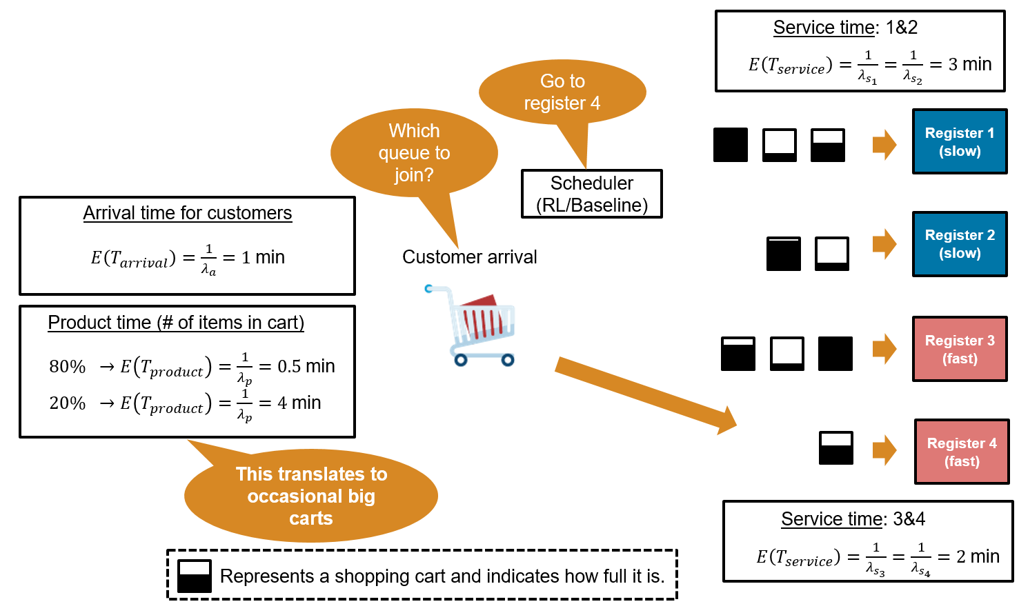
The system consists of four checkout registers, and the goal is to minimize customer waiting time by selecting the best queue for each arriving customer. The environment is as follows:

Customer Arrival: Customers arrive at the checkout area with exponentially distributed inter‑arrival times. The mean arrival time is 1 minute. Because the arrival rate parameter $λ_{a}$ is 1 customer per minute, the mean customer arrival time is = $\frac{1}{λ_{a}}$ = 1 minute:

$E (T_{a r r i v a l}) = \frac{1}{λ_{a}} = 1 m i n u t e$

Product Time (Cart Size): At generation, each customer is assigned a cart product time that represents the time needed to scan their items. The product time is drawn from an exponential distribution with two possible means: 80% of customers have a small cart with a mean of 0.5 min, and 20% have a large cart with a mean product time of 4 min.

$E (T_{p r o d u c t}) = \frac{1}{λ_{p s}} = 0.5 m i n u t e s$ (small carts, 80% of the time)

$E (T_{p r o d u c t}) = \frac{1}{λ_{p b}} = 4 m i n u t e s$ (big carts, 20% of the time)

Service Time (Registers): The checkout area consists of four registers, each with its own dedicated queue. Registers 1 and 2 are classified as slow, with exponentially distributed service times averaging 3 min, while registers 3 and 4 are fast, with service times averaging 2 min.

$E (T_{s e r v i c e}) = \frac{1}{λ_{s 1}} = \frac{1}{λ_{s 2}} = 3 m i n u t e s$ (slow lanes)

$E (T_{s e r v i c e}) = \frac{1}{λ_{s 3}} = \frac{1}{λ_{s 4}} = 2 m i n u t e s$ (fast lanes)

The total time a customer spends at a register is equal to the service time (which is register specific) plus the product time (which is cart specific). This means that a slow register with a big cart will take much longer than a fast register with a small cart.

Open the model.

mdl = "rlQueuingStrategiesModel";
open_system(mdl)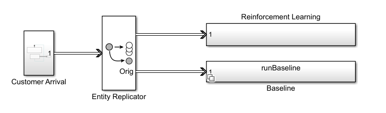

In this example, you model customer arrivals using the SimEvents Entity Generator block; see Entity Generator (SimEvents) for more information. The Entity Generator block assigns each customer a product time (cart size) at generation. To enable comparison between the reinforcement learning and the baseline strategies, the Entity Replicator block clones each generated customer, and then sends the same customer through both the RL and baseline strategies block. Each of the two strategy block routes the customer to one of the four queues. When a customer joins a queue, the corresponding queue block assigns the appropriate service time distribution based on the register type.

Open the reinforcement learning subsystem.

open_system(mdl+"/Reinforcement Learning")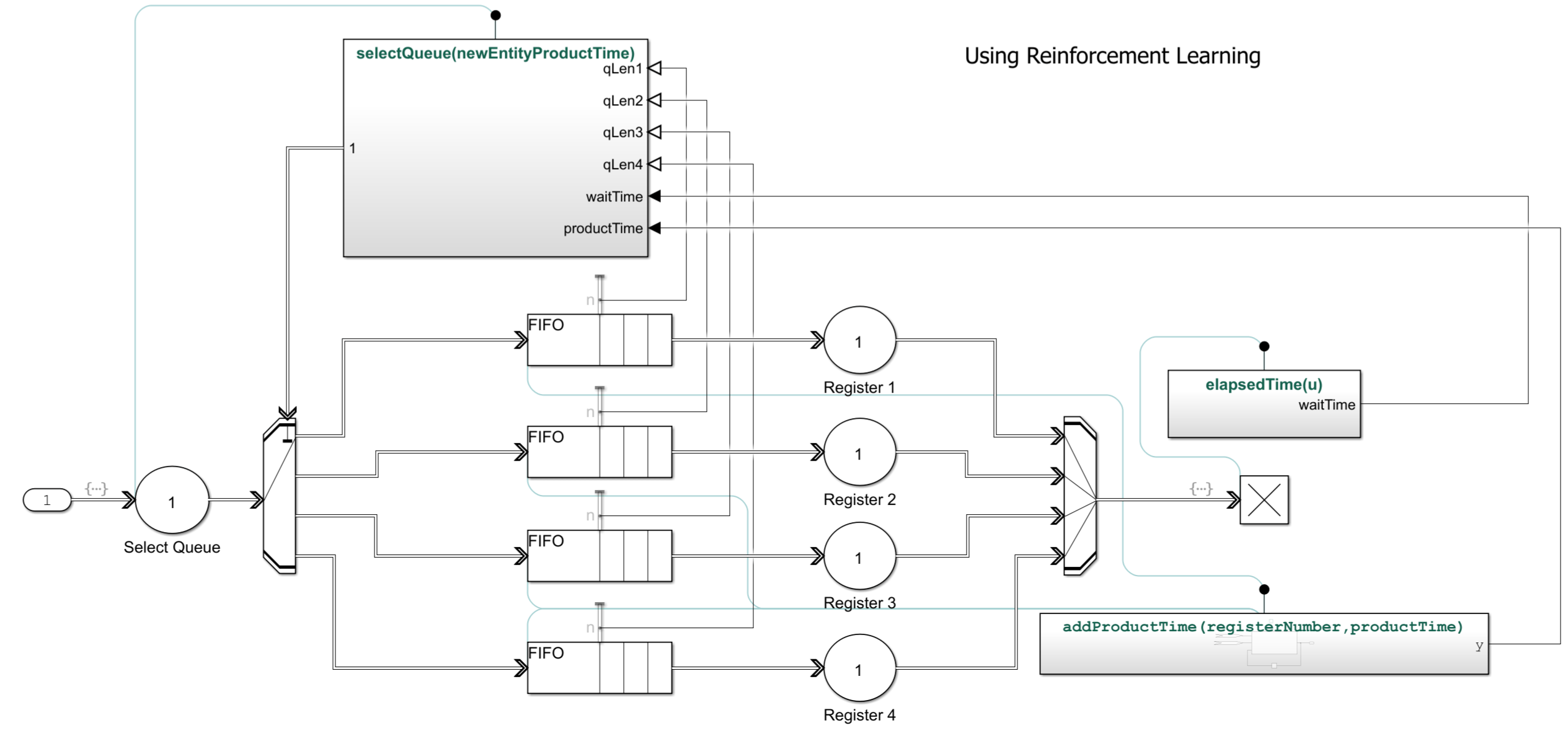

Open the Queue Selector block inside the Reinforcement Learning subsystem.

open_system(mdl+"/Reinforcement Learning/Queue Selector")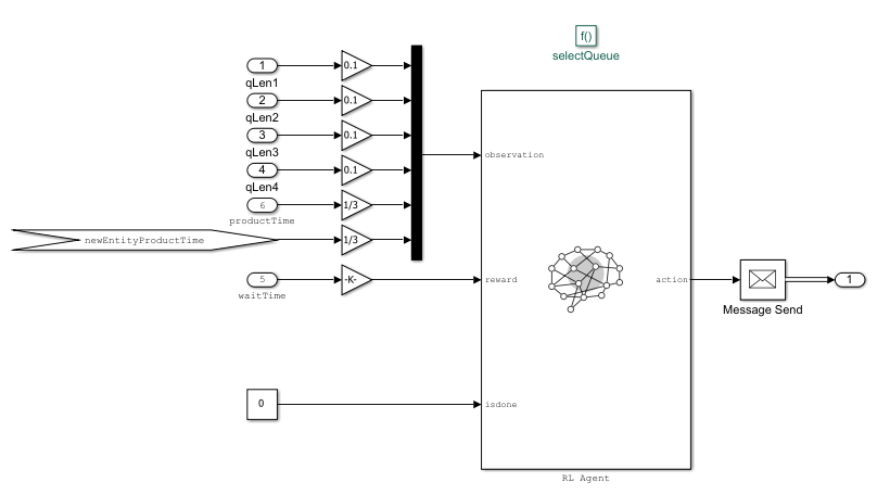

IIn this Simulink model:

The RL Agent block is inside the Queue Selector block.
The environment provides the following 9 observations to the RL Agent block: queue lengths for all 4 registers, total product time in each queue (proxy for number of items in carts), current customer's product time (cart size). Note that the agent does not have any prior knowledge of which registers are fast and which are slow.
The agent has a discrete action space consisting or the elements 1,2,3 and 4 corresponding to the which queue the arriving customer should join.
The reward is computed as the negative of the waiting time. The waiting time is measured from entity generation until the customer completes checkout at the register.

Baseline strategy: To evaluate performance, the RL agent is compared against a baseline heuristic strategy. The baseline aims to minimize estimated future workload by selecting the queue with the smallest product between the number of people waiting in line and the cumulative product time. It is implemented as a variant subsystem that remains disabled during training and is enabled during the simulation phase for comparison. You enable this strategy using the runBaseline workspace variable.

Create Environment Object

Define the observation specification obsInfo and the action specification actInfo.

obsInfo = rlNumericSpec([9 1]);
actInfo = rlFiniteSetSpec(1:4);

Use rlSimulinkEnv to create the environment object from the Simulink model, passing to it the path of the RL Agent block and the observation and action specification.

env = rlSimulinkEnv(mdl,mdl + "/Reinforcement Learning/Queue Selector/RL Agent",obsInfo,actInfo);

For more information about Simulink environments, see Create Custom Simulink Environments.

Create DQN Agent

When you create the agent, the initial parameters of the critic network are initialized with random values. Fix the random number stream so that the agent is always initialized with the same parameter values.

rng(0,"twister");

Create an agent initialization object to initialize the critic the network with a hidden layer size of 128.

initOptions = rlAgentInitializationOptions("NumHiddenUnit",128);

Create the DQN agent using the observation and action specifications and initialization options that you defined.

agent = rlDQNAgent(obsInfo,actInfo,initOptions);

Specify the agent options for training:

Specify the sample time as -1. Since this is an event-based simulation, you place the RL Agent block inside a conditionally executed subsystem. A SampleTime of -1 causes the block to inherit the sample time of its parent subsystem. For more information, see Conditionally Executed Subsystems Overview (Simulink).
Specify the discount factor of 0.9995. In this problem, the reward (negative customer waiting time) is delayed until service completes, so the agent must consider a longer sequence of actions before seeing the outcome. A high discount factor of 0.9995 ensures that the agent puts larger weight on future outcomes, enabling it to learn long-term strategies rather than making short-sighted decisions.
Specify the critic learning rate as 1e-3. A large learning rate may lead to divergent behaviors, while a low value may require learning rate might cause training to take longer.
Use a gradient threshold of 1 to clip the gradients. Clipping the gradients can improve training stability.
Use mini-batches of 128 experiences. Smaller mini-batches are computationally efficient, but might introduce variance in training. Larger batch sizes can make the training more stable but require more memory.
Specify the experience buffer length as 100 and number of epochs as 5. At each learning step, the agent samples up to MaxMiniBatchPerEpoch unique mini-batches per epoch.

agent.AgentOptions.SampleTime = -1;
agent.AgentOptions.DiscountFactor = 0.9995;
agent.AgentOptions.CriticOptimizerOptions.LearnRate = 1e-3;
agent.AgentOptions.CriticOptimizerOptions.GradientThreshold = 1;
agent.AgentOptions.MiniBatchSize = 128;
agent.AgentOptions.ExperienceBufferLength = 1e6;
agent.AgentOptions.NumEpoch = 5;

A DQN agent uses the epsilon-greedy algorithm to explore the action space during training. Specify a decay rate of 1e-4 for the epsilon value to gradually decay during training. The epsilon value is the probability that the agent will choose a random action instead of exploiting its current knowledge to maximize the reward. The gradual decay of the epsilon value during training promotes exploration toward the beginning of training when the agent does not have a good policy, and exploitation toward the end of training when the agent has learned the optimal policy.

agent.AgentOptions.EpsilonGreedyExploration.EpsilonDecay = 1e-4;
agent.AgentOptions.EpsilonGreedyExploration.EpsilonMin = 0.01;

For more information, see rlDQNAgentOptions.

Train DQN Agent

Fix the random stream for reproducibility.

rng(0,"twister");

Create an agent evaluator to evaluate the performance of the greedy policy every 25 training episodes.

rlEval = rlEvaluator("EvaluationFrequency",25,"NumEpisodes",1,"RandomSeeds",0);

To train the agent, first specify the training options. For this example, use the following options.

Run each training for a maximum of 300 episodes, with each episode lasting 1000 steps.
Display the training progress in the Reinforcement Learning Training Monitor dialog box (set the Plots option) and disable the command line display (set the Verbose option to false).
Set StopTrainingCriteria to "None" so that the training stops only when the number of episodes reaches MaxEpisodes.

For more information on training options, see rlTrainingOptions.

% Training options
trainOpts = rlTrainingOptions(...
    MaxEpisodes=300, ...
    MaxStepsPerEpisode=1000, ...
    Verbose=false, ...
    Plots="training-progress",...
    StopTrainingCriteria="EvaluationStatistic", ...
    StopTrainingValue=0);

Train the agent using the train function. Training this agent is a computationally intensive process that takes several minutes to complete. To save time while running this example, you can load a pretrained agent by setting doTraining to false. To train the agent yourself, set doTraining to true. The baseline controller is not needed during training, so set runBaseline to false.

doTraining = false;
runBaseline = false;
if doTraining
    % Train the agent.
    trainingStats = train(agent,env,trainOpts,Evaluator=rlEval);
else
    % Load the pretrained agent for the example.
    load("trainedAgentQueuingStrategies.mat","agent");
end

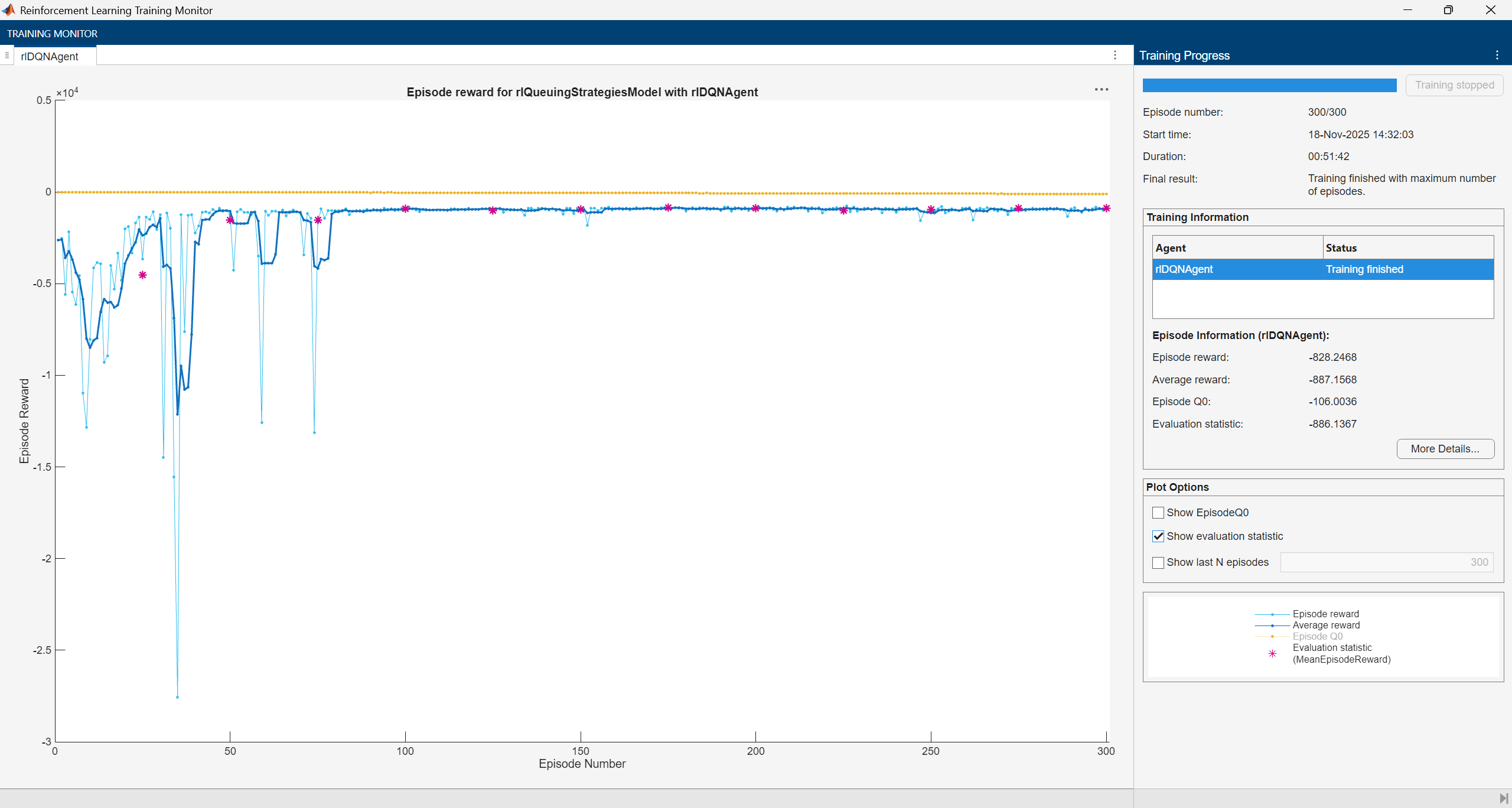
The training converges after 100 episodes.

Simulate DQN Agent

Fix the random stream for reproducibility.

rng(0,"twister");

Set runBaseline to true to enable the baseline controller and compare its performance against the RL agent.

runBaseline = true;

To validate the performance of the trained agent, simulate the trained agent with the environment. For more information on agent simulation, see rlSimulationOptions and sim.

agent.UseExplorationPolicy = false;
simOptions = rlSimulationOptions(MaxSteps=1000);
experience = sim(env,agent,simOptions);

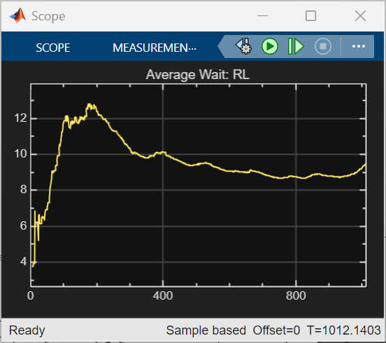
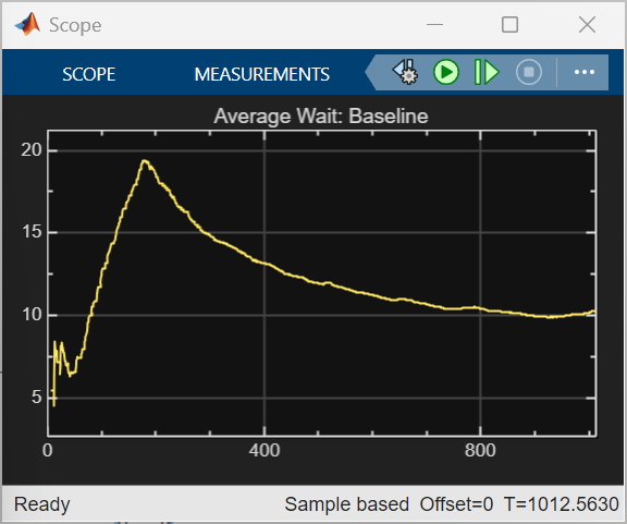
The trained RL agent achieves a lower total average waiting time of 9468 minutes, compared to 12150 minutes for the baseline strategy, showing better overall efficiency. RL also converges faster and maintains a lower average wait after the initial peak, while the baseline strategy exhibits higher peaks and slower recovery. These results reflect the current reward design. Alternative reward functions could combine minimizing average waiting time with constraints on maximum waiting time or queue length.

Understanding the Learned Policy

By comparing the agent’s decision with an intuitive heuristic (different from the baseline strategy), you can learn about its priorities, such as whether it minimizes immediate waiting time, protects fast lanes from large carts, or balances long-term efficiency. This is not an exhaustive validation, but a way to understand the strategies the policy has internalized.

To interpret what the RL agent has learned, examine its choices in representative scenarios. Each scenario is described by nine observations:

Number of people in each of the four queues
Total product time in each queue
Product time of the newly arrived customer

Define observations related to various scenarios.

obsScenarios = [
    0, 0, 0, 0, 0, 0, 0, 0, 1;
    0, 0, 0, 0, 0, 0, 0, 0, 8;
    2, 1, 0, 0, 15, 10, 0, 0, 8; 
    1, 0, 0, 1, 5, 0, 0, 6, 0.5; 
    1, 1, 2, 2, 5, 5, 1.5, 0.75, 0.5;
    1, 1, 2, 2, 4, 4, 8, 8, 0.5 ]';

Compute the action the trained agent takes in each of six different scenarios. In the Simulink model, observations are scaled before use. Therefore, scale the observations using the local function scaleObservations (defined at the end of the example) before feeding them to the trained agent to calculate the corresponding action.

actScenarios = getAction(agent,{scaleObservations(obsScenarios)});

Display the actions related to the six observations.

squeeze(actScenarios{:})'

ans = 1×6

     3     2     1     3     4     2

For each scenario, observations and actions are captured in the following table.

Scenario	Number of People in Each Queue	Total Product Time in Each Queue	New Customer's Product Time (Cart Size)	Intent/What to Look For	Expected Preference (Heuristic)	Actual Action (RL Policy)
1	0, 0, 0, 0	0, 0, 0, 0	1	Small cart, all queues empty	Send to fast lane (3 or 4)	3
2	0, 0, 0, 0	0, 0, 0, 0	8	Big cart, all queues empty	Send to slow lane (1 or 2)	2
3	2, 1, 0, 0	15, 10, 0, 0	8	Big cart, slow lanes are occupied and fast lanes are empty	Prefer slow lane (1 or 2) to avoid clogging fast lanes	1
4	1, 0, 0, 1	5, 0, 0, 6	0.5	Small cart, lane 4 has work	Send to lane 3 (fast and free)	3
5	1, 1, 2, 2	5, 5, 1.5, 0.75	0.5	All queues have work, small cart	Prefer fast lane with least load (3 or 4)	4
6	1, 1, 2, 2	4, 4, 8, 8	0.5	Small cart, fast lanes heavily loaded	Prefer slow lane (1 or 2) to minimize wait	2

Insights

Scenario 1: The agent sends a small cart to a fast lane when all queues are empty, which suggests that it values speed when there is no congestion.
Scenario 2: For a large cart with all queues empty, the agent chooses a slow lane, which might mean that the agent tries to keep fast lanes available for smaller carts.
Scenario 3: When slow lanes already have work and a large cart arrives, the agent still picks a slow lane, which again might mean that the it tries to protect fast lanes from heavy loads.
Scenario 4: With a small cart and lane 4 busy, the agent selects lane 3, which suggests that it considers both lane type and current load.
Scenario 5: When all queues have work and a small cart arrives, the agent prefers a fast lane, which could mean that it prioritizes minimizing expected waiting time even under congestion.
Scenario 6: When all queues have work and a small cart arrives, the agent chooses a slow lane instead of a fast lane. This suggests that the policy considers overall queue congestion and may route a small cart to a slower register if the fast lanes are heavily loaded, demonstrating a balance between lane speed and current load.

This analysis reveals that the policy has learned sensible strategies, such as sending small carts to fast lanes, large carts to slow lanes, and balancing queue load when possible. The agent also seems to have identified which registers are fast and which are slow from experience, without being explicitly told this information.

Restore the random number stream using the information stored in previousRngState.

rng(previousRngState);

Scale Observations Function

The scaleObservations functions scales the observations.

function scaledObs = scaleObservations(obsMatrix)
    % obsMatrix: 9xN matrix where each column is [q1 q2 q3 q4 p1 p2 p3 p4 pc]
    % First 4 rows scaled by 0.1
    % Next 5 rows scaled by 1/3
    
    [rows,~] = size(obsMatrix);
    if rows ~= 9
        error('Input must have 9 rows.');
    end
    
    scaledObs = obsMatrix; % copy original
    scaledObs(1:4,:) = obsMatrix(1:4,:)*0.1;   % scale first 4 rows
    scaledObs(5:9,:) = obsMatrix(5:9,:)*(1/3); % scale next 5 rows
end

Optimizing Queue Selection Strategies Using Reinforcement Learning

Fix Random Number Stream for Reproducibility

Environment Setup

Create Environment Object

Create DQN Agent

Train DQN Agent

Simulate DQN Agent

Understanding the Learned Policy

Scale Observations Function

See Also

Functions

Objects

Blocks

Topics