Bias Mitigation in Credit Scoring by Disparate Impact Removal

Open Live Script

Disparate impact removal is a pre-processing technique in bias mitigation. Using this technique, you modify the original credit score data to increase group fairness, while still preserving rank ordering within groups. Using a disparate impact removal technique reduces the bias introduced by the credit scoring model more than if you use the original data to train the credit scoring model. You perform the disparate impact removal technique using the disparateImpactRemover class from the Statistics and Machine Learning Toolbox™. This class returns a remover object along with a table containing the new predictor values. However, you need to use the transform method with the remover object on the test data before you can predict using the fitted credit scoring model.

The disparate impact removal technique works only with the distribution of data within a numeric predictor for each subgroup of a sensitive attribute. The disparateImpactRemover class has no knowledge of, or relation to, the response variable. In this example, you treat all the numeric predictors, time at address (TmAtAddress), customer income (CustIncome), time with Bank (TmWBank), average monthly balance (AMBalance), and utilization rate (UtilRate), with respect to the sensitive attribute, customer age (AgeGroup).

Original Credit Scoring Model

This example uses a credit scoring workflow. Load the CreditCardData.mat and use the 'data' data set.

load CreditCardData.mat

AgeGroup = discretize(data.CustAge,[min(data.CustAge) 30 45 60 max(data.CustAge)], ...
    'categorical',{'Age < 30','30 <= Age < 45','45 <= Age < 60','Age >= 60'});
data = addvars(data,AgeGroup,'After','CustAge');
head(data)

    CustID    CustAge       AgeGroup       TmAtAddress    ResStatus     EmpStatus    CustIncome    TmWBank    OtherCC    AMBalance    UtilRate    status
    ______    _______    ______________    ___________    __________    _________    __________    _______    _______    _________    ________    ______

      1         53       45 <= Age < 60        62         Tenant        Unknown        50000         55         Yes       1055.9        0.22        0   
      2         61       Age >= 60             22         Home Owner    Employed       52000         25         Yes       1161.6        0.24        0   
      3         47       45 <= Age < 60        30         Tenant        Employed       37000         61         No        877.23        0.29        0   
      4         50       45 <= Age < 60        75         Home Owner    Employed       53000         20         Yes       157.37        0.08        0   
      5         68       Age >= 60             56         Home Owner    Employed       53000         14         Yes       561.84        0.11        0   
      6         65       Age >= 60             13         Home Owner    Employed       48000         59         Yes       968.18        0.15        0   
      7         34       30 <= Age < 45        32         Home Owner    Unknown        32000         26         Yes       717.82        0.02        1   
      8         50       45 <= Age < 60        57         Other         Employed       51000         33         No        3041.2        0.13        0

rng('default')

Split the data set into training and testing data.

c = cvpartition(size(data,1),'HoldOut',0.3);
data_Train = data(c.training(),:);
data_Test = data(c.test(),:);
head(data_Train)

    CustID    CustAge       AgeGroup       TmAtAddress    ResStatus     EmpStatus    CustIncome    TmWBank    OtherCC    AMBalance    UtilRate    status
    ______    _______    ______________    ___________    __________    _________    __________    _______    _______    _________    ________    ______

       1        53       45 <= Age < 60        62         Tenant        Unknown        50000         55         Yes       1055.9        0.22        0   
       2        61       Age >= 60             22         Home Owner    Employed       52000         25         Yes       1161.6        0.24        0   
       3        47       45 <= Age < 60        30         Tenant        Employed       37000         61         No        877.23        0.29        0   
       4        50       45 <= Age < 60        75         Home Owner    Employed       53000         20         Yes       157.37        0.08        0   
       7        34       30 <= Age < 45        32         Home Owner    Unknown        32000         26         Yes       717.82        0.02        1   
       8        50       45 <= Age < 60        57         Other         Employed       51000         33         No        3041.2        0.13        0   
       9        50       45 <= Age < 60        10         Tenant        Unknown        52000         25         Yes       115.56        0.02        1   
      10        49       45 <= Age < 60        30         Home Owner    Unknown        53000         23         Yes        718.5        0.17        1

Use creditscorecard to create a creditscorecard object and use fitmodel to fit a credit scoring model with the training data (data_Train).

PredictorVars = setdiff(data_Train.Properties.VariableNames, ...
    {'CustAge','AgeGroup','CustID','status'});
sc1 = creditscorecard(data_Train,'IDVar','CustID', ...
    'PredictorVars',PredictorVars,'ResponseVar','status');
sc1 = autobinning(sc1);
sc1 = fitmodel(sc1,'VariableSelection','fullmodel');

Generalized linear regression model:
    logit(status) ~ 1 + TmAtAddress + ResStatus + EmpStatus + CustIncome + TmWBank + OtherCC + AMBalance + UtilRate
    Distribution = Binomial

Estimated Coefficients:
                   Estimate       SE        tStat        pValue  
                   ________    ________    ________    __________

    (Intercept)     0.73924    0.077237      9.5711     1.058e-21
    TmAtAddress      1.2577     0.99118      1.2689       0.20448
    ResStatus         1.755       1.295      1.3552       0.17535
    EmpStatus       0.88652     0.32232      2.7504     0.0059516
    CustIncome      0.95991     0.19645      4.8862    1.0281e-06
    TmWBank           1.132      0.3157      3.5856    0.00033637
    OtherCC         0.85227      2.1198     0.40204       0.68765
    AMBalance        1.0773     0.31969      3.3698    0.00075232
    UtilRate       -0.19784     0.59565    -0.33214       0.73978


840 observations, 831 error degrees of freedom
Dispersion: 1
Chi^2-statistic vs. constant model: 66.5, p-value = 2.44e-11

Use displaypoints to compute the points per predictor per bin for the creditscorecard model (sc1).

pointsinfo1 = displaypoints(sc1)

pointsinfo1=38×3 table
      Predictors              Bin            Points  
    _______________    _________________    _________

    {'TmAtAddress'}    {'[-Inf,9)'     }     -0.17538
    {'TmAtAddress'}    {'[9,16)'       }      0.05434
    {'TmAtAddress'}    {'[16,23)'      }     0.096897
    {'TmAtAddress'}    {'[23,Inf]'     }      0.13984
    {'TmAtAddress'}    {'<missing>'    }          NaN
    {'ResStatus'  }    {'Tenant'       }    -0.017688
    {'ResStatus'  }    {'Home Owner'   }      0.11681
    {'ResStatus'  }    {'Other'        }      0.29011
    {'ResStatus'  }    {'<missing>'    }          NaN
    {'EmpStatus'  }    {'Unknown'      }    -0.097582
    {'EmpStatus'  }    {'Employed'     }      0.33162
    {'EmpStatus'  }    {'<missing>'    }          NaN
    {'CustIncome' }    {'[-Inf,30000)' }     -0.61962
    {'CustIncome' }    {'[30000,36000)'}     -0.10695
    {'CustIncome' }    {'[36000,40000)'}    0.0010845
    {'CustIncome' }    {'[40000,42000)'}     0.065532
      ⋮

Use probdefault to determine the likelihood of default for the data_Test data set and the creditscorecard model (sc1).

pd1 = probdefault(sc1,data_Test);
threshold = 0.35;
predictions1 = double(pd1>threshold);

Use fairnessMetrics to compute fairness metrics at the model level as a baseline. Use report to generate the fairness metrics report.

modelMetrics1 = fairnessMetrics(data_Test,'status','Predictions',predictions1,'SensitiveAttributeNames','AgeGroup'); 
mmReport1 = report(modelMetrics1,'GroupMetrics','GroupCount')

mmReport1=4×8 table
    ModelNames    SensitiveAttributeNames        Groups        StatisticalParityDifference    DisparateImpact    EqualOpportunityDifference    AverageAbsoluteOddsDifference    GroupCount
    __________    _______________________    ______________    ___________________________    _______________    __________________________    _____________________________    __________

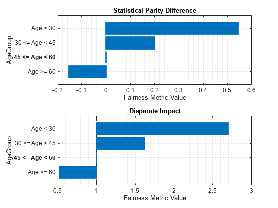
      Model1             AgeGroup            Age < 30                    0.54312                  2.6945                   0.47391                         0.5362                   22    
      Model1             AgeGroup            30 <= Age < 45              0.19922                  1.6216                   0.35645                        0.22138                  152    
      Model1             AgeGroup            45 <= Age < 60                    0                       1                         0                              0                  156    
      Model1             AgeGroup            Age >= 60                  -0.15385                    0.52                  -0.18323                        0.16375                   30

Use plot to visualize the statistical parity difference ('spd') and disparate impact ('di') bias metrics.

figure
tiledlayout(2,1)
nexttile
plot(modelMetrics1,'spd')
nexttile
plot(modelMetrics1,'di')

Figure contains 2 axes objects. Axes object 1 with title Statistical Parity Difference, xlabel Fairness Metric Value, ylabel AgeGroup contains an object of type bar. Axes object 2 with title Disparate Impact, xlabel Fairness Metric Value, ylabel AgeGroup contains an object of type bar.

Bias Mitigation by Disparate Impact Removal

For each of the five continuous predictors, 'TmAtAddress', 'CustIncome', 'TmWBank', 'AMBalance', and 'UtilRate' plot the original distributions of data within each age group.

Choose a numeric predictor to plot.

predictor = "CustIncome";
[f1, xi1] = ksdensity(data_Train.(predictor)(data_Train.AgeGroup=='Age < 30'));
[f2, xi2] = ksdensity(data_Train.(predictor)(data_Train.AgeGroup=='30 <= Age < 45'));
[f3, xi3] = ksdensity(data_Train.(predictor)(data_Train.AgeGroup=='45 <= Age < 60'));
[f4, xi4] = ksdensity(data_Train.(predictor)(data_Train.AgeGroup=='Age >= 60'));

Create a disparateImpactRemover object and return the newTrainTbl table with the new predictor values.

[remover, newTrainTbl] = disparateImpactRemover(data_Train, 'AgeGroup' , 'PredictorNames', {'TmAtAddress','CustIncome','TmWBank','AMBalance','UtilRate'})

remover = 
  disparateImpactRemover with properties:

        RepairFraction: 1
        PredictorNames: {'TmAtAddress'  'CustIncome'  'TmWBank'  'AMBalance'  'UtilRate'}
    SensitiveAttribute: 'AgeGroup'

newTrainTbl=840×12 table
    CustID    CustAge       AgeGroup       TmAtAddress    ResStatus     EmpStatus    CustIncome    TmWBank    OtherCC    AMBalance    UtilRate    status
    ______    _______    ______________    ___________    __________    _________    __________    _______    _______    _________    ________    ______

       1        53       45 <= Age < 60      58.599       Tenant        Unknown        47000       51.733       Yes       1009.4       0.20099      0   
       2        61       Age >= 60               24       Home Owner    Employed       41500         24.5       Yes       1203.9          0.25      0   
       3        47       45 <= Age < 60        30.5       Tenant        Employed       33500       57.686       No         817.9          0.29      0   
       4        50       45 <= Age < 60      68.622       Home Owner    Employed       49401        19.07       Yes       120.54      0.077267      0   
       7        34       30 <= Age < 45        30.5       Home Owner    Unknown        35500       26.657       Yes       638.88          0.02      1   
       8        50       45 <= Age < 60       53.39       Other         Employed       47000       27.971       No        2172.7          0.12      0   
       9        50       45 <= Age < 60           9       Tenant        Unknown        49401       22.541       Yes       120.54          0.02      1   
      10        49       45 <= Age < 60        30.5       Home Owner    Unknown        49401           22       Yes       664.51       0.14715      1   
      11        52       45 <= Age < 60          24       Tenant        Unknown        30500       38.779       Yes       120.54         0.065      1   
      12        48       45 <= Age < 60      77.291       Other         Unknown        40500         14.5       Yes       405.81          0.03      0   
      14        44       30 <= Age < 45      68.622       Other         Unknown        44500       34.791       No        378.88       0.15657      0   
      17        39       30 <= Age < 45           9       Tenant        Employed       37500       38.779       Yes       664.51          0.25      1   
      20        52       45 <= Age < 60      51.442       Other         Unknown        38500       12.297       Yes       1157.5       0.19273      0   
      21        37       30 <= Age < 45      10.343       Tenant        Unknown        36500       23.314       No        732.28         0.065      1   
      22        51       45 <= Age < 60      12.087       Home Owner    Employed       31500       27.971       Yes       437.95          0.01      0   
      24        43       30 <= Age < 45          40       Tenant        Employed       33500        11.18       Yes       263.13      0.077267      0   
      ⋮

[nf1, nxi1] = ksdensity(newTrainTbl.(predictor)(newTrainTbl.AgeGroup=='Age < 30'));
[nf2, nxi2] = ksdensity(newTrainTbl.(predictor)(newTrainTbl.AgeGroup=='30 <= Age < 45'));
[nf3, nxi3] = ksdensity(newTrainTbl.(predictor)(newTrainTbl.AgeGroup=='45 <= Age < 60'));
[nf4, nxi4] = ksdensity(newTrainTbl.(predictor)(newTrainTbl.AgeGroup=='Age >= 60'));

Plot the original and the repaired distributions.

figure;
tiledlayout(2,1)
ax1 = nexttile;
plot(xi1, f1, 'LineWidth', 1.5)
hold on
plot(xi2, f2, 'LineWidth', 1.5)
plot(xi3, f3, 'LineWidth', 1.5)
plot(xi4, f4, 'LineWidth', 1.5)
legend(["Age < 30"; "30 <= Age < 45"; "45 <= Age < 60"; "Age >= 60"],'Location','northwest')
ax1.Title.String = "Original Distribution of " + predictor;
xlabel(predictor)
ylabel('pdf')
grid on
ax2 = nexttile;
plot(nxi1, nf1, 'LineWidth', 1.5)
hold on
plot(nxi2, nf2, 'LineWidth', 1.5)
plot(nxi3, nf3, 'LineWidth', 1.5)
plot(nxi4, nf4, 'LineWidth', 1.5)
legend(["Age < 30"; "30 <= Age < 45"; "45 <= Age < 60"; "Age >= 60"],'Location','northwest')
ax2.Title.String = "Repaired Distribution of " + predictor;
xlabel(predictor)
ylabel('pdf')
grid on
linkaxes([ax1, ax2], 'xy')

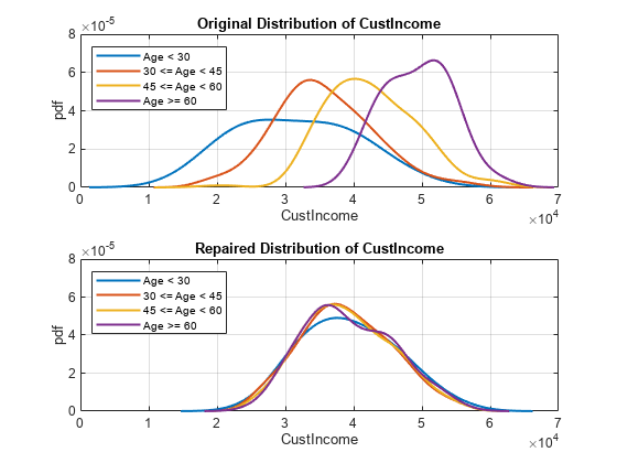
This plot demonstrates that the initial distributions of CustIncome of each group within the AgeGroup predictor are different. Younger people seem to have a lower income on average and more variation than older people. This difference introduces bias, which the fitted model then reflects. The disparateImpactRemover function modifies the data so that the distributions of all the subgroups are more similar. You see this distribution in the second subplot Repaired Distribution of CustIncome. Using this new data, you can fit a logistic regression model and then measure the model-level metrics and compare these with the model-level metrics from the original creditscorecard model (sc1).

New Credit Scoring Model

Use creditscorecard to create a creditscorecard object and use fitmodel to fit a credit scoring model with the new data (newTrainTbl). Then, you can compute model-level bias metrics using fairnessMetrics.

sc2 = creditscorecard(newTrainTbl,'IDVar','CustID', ...
      'PredictorVars',PredictorVars,'ResponseVar','status');
sc2 = autobinning(sc2);
sc2 = fitmodel(sc2,'VariableSelection','fullmodel');

Generalized linear regression model:
    logit(status) ~ 1 + TmAtAddress + ResStatus + EmpStatus + CustIncome + TmWBank + OtherCC + AMBalance + UtilRate
    Distribution = Binomial

Estimated Coefficients:
                   Estimate       SE        tStat       pValue  
                   _________    _______    _______    __________

    (Intercept)      0.74041    0.07641     9.6899     3.327e-22
    TmAtAddress       1.1658    0.87564     1.3313       0.18308
    ResStatus         1.8719     1.2848     1.4569       0.14513
    EmpStatus        0.88699    0.31991     2.7727       0.00556
    CustIncome       0.98269    0.28725      3.421    0.00062396
    TmWBank           1.1392    0.30677     3.7135    0.00020442
    OtherCC          0.55005     2.0969    0.26231       0.79308
    AMBalance         1.0478     0.3607     2.9049     0.0036734
    UtilRate       -0.071972    0.58704    -0.1226       0.90242


840 observations, 831 error degrees of freedom
Dispersion: 1
Chi^2-statistic vs. constant model: 50.4, p-value = 3.36e-08

Use displaypoints to compute the points per predictor per bin for the creditscorecard model (sc2).

pointsinfo2 = displaypoints(sc2)

pointsinfo2=35×3 table
      Predictors              Bin            Points  
    _______________    _________________    _________

    {'TmAtAddress'}    {'[-Inf,9)'     }     -0.11003
    {'TmAtAddress'}    {'[9,15.1453)'  }    -0.091424
    {'TmAtAddress'}    {'[15.1453,Inf]'}      0.14546
    {'TmAtAddress'}    {'<missing>'    }          NaN
    {'ResStatus'  }    {'Tenant'       }    -0.024878
    {'ResStatus'  }    {'Home Owner'   }      0.11858
    {'ResStatus'  }    {'Other'        }      0.30343
    {'ResStatus'  }    {'<missing>'    }          NaN
    {'EmpStatus'  }    {'Unknown'      }    -0.097539
    {'EmpStatus'  }    {'Employed'     }       0.3319
    {'EmpStatus'  }    {'<missing>'    }          NaN
    {'CustIncome' }    {'[-Inf,31500)' }     -0.30942
    {'CustIncome' }    {'[31500,38500)'}     -0.09789
    {'CustIncome' }    {'[38500,45000)'}      0.21233
    {'CustIncome' }    {'[45000,Inf]'  }        0.494
    {'CustIncome' }    {'<missing>'    }          NaN
      ⋮

Before computing probabilities of default with the test data, you need to transform the test data using the same transformation as for the training data. To make this transformation, use the transform method of the remover object and pass it in the data_Test data set. Then, use probdefault to compute the likelihood of default of the data_Test data set.

newTestTbl = transform(remover,data_Test);
pd2 = probdefault(sc2,newTestTbl);
predictions2 = double(pd2>threshold);

Use fairnessMetrics to compute fairness metrics at the model level and use report to generate a fairness metrics report.

modelMetrics2 = fairnessMetrics(newTestTbl,'status','Predictions',predictions2,'SensitiveAttributeNames','AgeGroup'); 
mmReport2 = report(modelMetrics2,'GroupMetrics','GroupCount')

mmReport2=4×8 table
    ModelNames    SensitiveAttributeNames        Groups        StatisticalParityDifference    DisparateImpact    EqualOpportunityDifference    AverageAbsoluteOddsDifference    GroupCount
    __________    _______________________    ______________    ___________________________    _______________    __________________________    _____________________________    __________

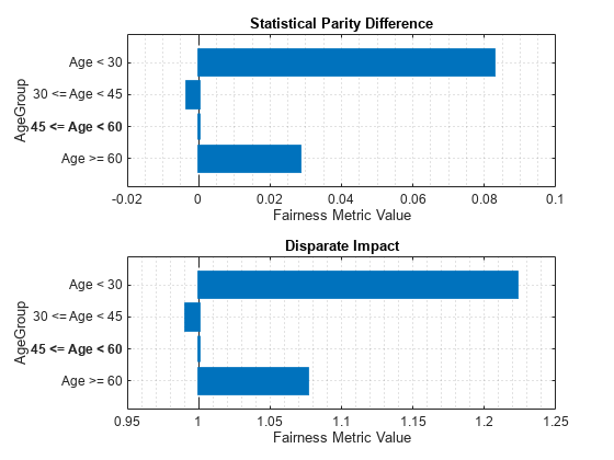
      Model1             AgeGroup            Age < 30                    0.082751                  1.2226                  0.18696                        0.10408                   22    
      Model1             AgeGroup            30 <= Age < 45            -0.0033738                 0.99093                  0.07902                       0.076333                  152    
      Model1             AgeGroup            45 <= Age < 60                     0                       1                        0                              0                  156    
      Model1             AgeGroup            Age >= 60                   0.028205                  1.0759                 0.015528                       0.026143                   30

Use plot to visualize the statistical parity difference ('spd') and disparate impact ('di') bias metrics.

figure
tiledlayout(2,1)
nexttile
plot(modelMetrics2,'spd')
nexttile
plot(modelMetrics2,'di')

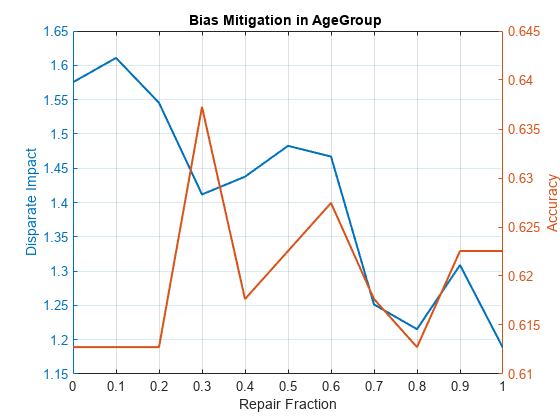
Plot Disparate Impact and Accuracy for Different Repair Fraction Values

In this example, the bias mitigation process uses disparateImpactRemover to set RepairFraction = 1 in order to mitigate bias. However, it is useful to see how the disparate impact and accuracy varies with a change in the RepairFraction value. For example, use the AgeGroup predictor and plot the disparate impact and accuracy of the different subgroups for different values of RepairFraction.

subgroup = 4;
r = 0:0.1:1;
Accuracy = zeros(11,1);
di = zeros(11,1);

for i = 0:1:10
    [rmvr, trainTbl] = disparateImpactRemover(data_Train, 'AgeGroup' , ...
           'PredictorNames', {'TmAtAddress','CustIncome','TmWBank','AMBalance','UtilRate'},'RepairFraction',i/10);
    testTbl = transform(rmvr, data_Test);
    sc = creditscorecard(trainTbl,'IDVar','CustID', ...
        'PredictorVars',PredictorVars,'ResponseVar','status');
    sc = autobinning(sc);
    sc = fitmodel(sc,'VariableSelection','fullmodel','Display','off');
    pd = probdefault(sc,testTbl);
    predictions = double(pd>threshold);
    modelMetrics = fairnessMetrics(newTestTbl, 'status', 'Predictions', predictions, 'SensitiveAttributeNames','AgeGroup'); 
    mmReport = report(modelMetrics,'BiasMetrics','di','GroupMetrics','accuracy');
    di(i+1) = mmReport.DisparateImpact(subgroup);
    Accuracy(i+1) = mmReport.Accuracy(subgroup);
end

figure
yyaxis left
plot(r, di,'LineWidth', 1.5)
title('Bias Mitigation in AgeGroup ')
xlabel('Repair Fraction')
ylabel('Disparate Impact')
yyaxis right
plot(r, Accuracy,'LineWidth', 1.5)
ylabel('Accuracy')
grid on

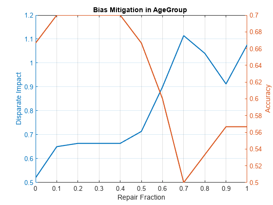
Figure contains an axes object. The axes object with title Bias Mitigation in AgeGroup, xlabel Repair Fraction, ylabel Accuracy contains 2 objects of type line.

If you select the subgroup 'Age < 30' from this plot, you can see that the accuracy increases as the RepairFraction value increases. Although this seems counterintuitive, looking further at the GroupCount of that age group in the mmReport2 table, this group has only 22 observations. This small number of observations explains the anomaly in this plot.

One way to mitigate this issue of not having enough data for a subgroup is to combine all unprivileged groups and compare them as one group against the privileged group. The following code shows you how by setting the majority group (45 <= Age < 60) as the privileged group and then by combining every other group into one and setting that group as the unprivileged group.

privilegedGroup = '45 <= Age < 60';
twoAgeGroups_TrainTbl = data_Train;
twoAgeGroups_TrainTbl.AgeGroup = addcats(twoAgeGroups_TrainTbl.AgeGroup,'Other','After','Age >= 60');
twoAgeGroups_TrainTbl.AgeGroup(twoAgeGroups_TrainTbl.AgeGroup ~= privilegedGroup) = 'Other';
twoAgeGroups_TestTbl = data_Test;
twoAgeGroups_TestTbl.AgeGroup = addcats(twoAgeGroups_TestTbl.AgeGroup,'Other','After','Age >= 60');
twoAgeGroups_TestTbl.AgeGroup(twoAgeGroups_TestTbl.AgeGroup ~= privilegedGroup) = 'Other';

r = 0:0.1:1;
Accuracy = zeros(11,1);
di = zeros(11,1);

for i = 0:1:10
  [rmvr, trainTbl] = disparateImpactRemover(twoAgeGroups_TrainTbl, 'AgeGroup' , ...
          'PredictorNames', {'TmAtAddress','CustIncome','TmWBank','AMBalance','UtilRate'},'RepairFraction',i/10);
   testTbl = transform(rmvr, twoAgeGroups_TestTbl);
   sc = creditscorecard(trainTbl,'IDVar','CustID', ...
          'PredictorVars',PredictorVars,'ResponseVar','status');
   sc = autobinning(sc);
   sc = fitmodel(sc,'VariableSelection','fullmodel','Display','off');
   pd = probdefault(sc,testTbl);
   predictions = double(pd>threshold);
   modelMetrics = fairnessMetrics(twoAgeGroups_TestTbl, 'status', 'Predictions', predictions, ...
        'SensitiveAttributeNames','AgeGroup','ReferenceGroup','45 <= Age < 60'); 
    mmReport = report(modelMetrics,'BiasMetrics','di','GroupMetrics','accuracy');
    di(i+1) = mmReport.DisparateImpact(2);
    Accuracy(i+1) = mmReport.Accuracy(2);
end

figure
yyaxis left
plot(r, di,'LineWidth', 1.5)
title('Bias Mitigation in AgeGroup ')
xlabel('Repair Fraction')
ylabel('Disparate Impact')
yyaxis right
plot(r, Accuracy,'LineWidth', 1.5)
ylabel('Accuracy')
grid on

Figure contains an axes object. The axes object with title Bias Mitigation in AgeGroup, xlabel Repair Fraction, ylabel Accuracy contains 2 objects of type line.

You can use this privileged group and unprivileged group method if the goal is not to measure the bias of each individual group against the privileged group, but rather to measure the overall fairness of all customers who are not part of the privileged group.

References

[1] Nielsen, Aileen. "Chapter 4. Fairness PreProcessing." Practical Fairness. O'Reilly Media, Inc., Dec. 2020.

[2] Mehrabi, Ninareh, et al. “A Survey on Bias and Fairness in Machine Learning.” ArXiv:1908.09635 [Cs], Sept. 2019. arXiv.org, https://arxiv.org/abs/1908.09635.

[3] Wachter, Sandra, et al. Bias Preservation in Machine Learning: The Legality of Fairness Metrics Under EU Non-Discrimination Law. SSRN Scholarly Paper, ID 3792772, Social Science Research Network, 15 Jan. 2021. papers.ssrn.com, https://papers.ssrn.com/sol3/papers.cfm?abstract_id=3792772.