Common Binning Explorer Tasks
The Binning Explorer app supports the following tasks:
Import Data
Binning Explorer enables you to import data by either
starting directly from the data stored in a MATLAB® table or by
loading an existing creditscorecard object.
Clean Start from Data
To start directly from data:
Place the credit scorecard data in your MATLAB workspace. The data must be in a MATLAB table, where each column of data can be any one of the following data types:
Numeric
Logical
Cell array of character vectors
Character array
Categorical
In addition, the table must contain a binary response variable.
Open Binning Explorer from the MATLAB toolstrip: On the Apps tab, under Computational Finance, click the app icon.
Click Import Data and select the data from the Step 1 pane of the Import Data window.
From the Step 2 pane, set the Variable Type for each of the predictors, as needed. If the input MATLAB table contains a column for
weights, from the Step 2 pane, using the Variable Type column, click the drop-down to select Weights. If the data contains missing values, from the Step 2 pane, set Bin missing data to Yes. For more information on working with missing data, see Credit Scorecard Modeling with Missing Values.From the Step 3 pane, select an initial binning algorithm and click Import Data. The bins are plotted and displayed for each predictor. By clicking an individual predictor plot in the Overview pane, the details for that predictor plot display in the main pane with additional information in the Bin Information and Predictor Information panes.
Start from an Existing creditscorecard Object
To start using an existing creditscorecard object:
Place the
creditscorecardobject in your MATLAB workspace. Create thecreditscorecardobject either by usingcreditscorecardor by clicking Export in the Binning Explorer to export and save acreditscorecardobject to the MATLAB workspace.Open Binning Explorer from the MATLAB toolstrip: On the Apps tab, under Computational Finance, click the app icon.
Click Import Data and from Step 1 pane of the Import Data window, select the
creditscorecardobject.From the Step 3 pane, select a binning algorithm. When using an existing
creditscorecardobject, it is recommended to select the No Binning option. To display the predictor plots, click Import Data.The bins are plotted and displayed for each predictor. By clicking an individual predictor plot in the Overview pane, the predictor plot displays in the main pane and associated information displays in the Bin Information and Predictor Information panes.
Start from MATLAB Command Line Using Data or an Existing creditscorecard Object
To start Binning Explorer from the MATLAB command line:
Place the credit scorecard data or existing
creditscorecardobject in your MATLAB workspace.At the MATLAB command prompt:
Enter
binningExplorer(data)orbinningExplorer(data,Name,Value)to open a table in the Binning Explorer app by specifying a table (data) as input.Enter
binningExplorer(sc)to open an existingcreditscorecardobject in the Binning Explorer app by specifying acreditscorecardobject (sc) as input.
The bins are plotted and displayed for each predictor. By clicking an individual predictor plot in the Overview pane, the details for that predictor plot display in the main pane and the associated details display in the Bin Information and Predictor Information panes.
Change Predictor Type
After you import data or a creditscorecard object
into Binning Explorer, you can change the predictor type.
Click any predictor plot. The name of the selected predictor displays on the Binning Explorer toolstrip under Selected Predictor.
On the Binning Explorer toolstrip, the predictor type for the selected predictor displays under Predictor Type.
To change the predictor type, under Predictor Type, select:
Numeric,Categorical, orOrdinal. The predictor plot is updated and the details in the Bin Information and Predictor Information panes are also updated.
Change Binning Algorithm for One or More Predictors
After you import data or a creditscorecard object
into Binning Explorer, you can change the binning algorithm
for an individual predictor or for multiple predictors.
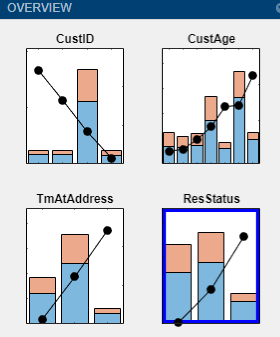
Click any predictor plot in the Overview pane. The selected predictor plot displays in the main pane.
Tip
When you select a predictor plot, a status message appears above Bin Information that displays the last binning information for that predictor. Use this information to determine which binning algorithm is most recently applied to an individual predictor plot.
On the Binning Explorer toolstrip, click to select Monotone, Split, Merge, Equal Frequency, or Equal Width. The predictor plot is updated with a change of algorithm. The details in the Bin Information and Predictor Information panes are also updated.
To change the binning algorithm for multiple predictors, multiselect more than one predictor plot by using Ctrl + click or Shift + click to highlight each predictor plot with a blue outline.
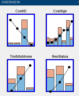
Click to select Monotone, Split, Merge, Equal Frequency, or Equal Width. All the selected predictor plots are updated for a change of algorithm.
Change Algorithm Options for Binning Algorithms
After you import data or a creditscorecard object into Binning
Explorer, you can change the binning algorithm options for an individual
predictor or for multiple predictors.
Click any predictor plot in the Overview pane. The predictor plot displays with a blue outline and displays in the main pane.

Tip
When you select a predictor plot with the blue outline, a status message appears above Bin Information that displays the last binning information for that predictor. Use this information to determine which binning algorithm is most recently applied to an individual predictor plot.
On the Binning Explorer toolstrip, click Options to open a list of options for the Monotone, Split, Merge, Equal Frequency, and Equal Width algorithms. Click an option to open the associated Algorithm options dialog box. For example, clicking Monotone Options opens the Algorithm options dialog box for Monotone.
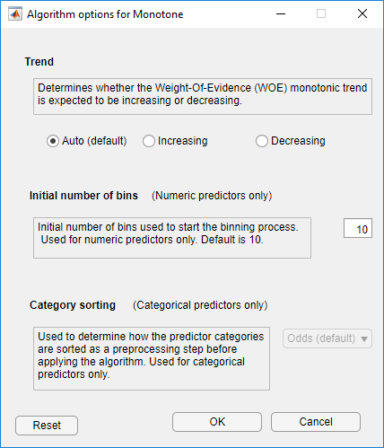
From the associated Algorithm options dialog box:
Monotone
For Trend, select one of the following:
Auto (default) — Automatically determines if the WOE trend is increasing or decreasing.
Increasing — Looks for an increasing WOE trend.
Decreasing — Looks for a decreasing WOE trend.
The value of Trend does not necessarily reflect that of the resulting WOE curve. The Trend option tells the algorithm to look for an increasing or decreasing trend, but the outcome might not show the desired trend. For example, the algorithm cannot find a decreasing trend when the data actually has an increasing WOE trend. For more information on the Trend option, see Monotone.
For Initial number of bins, enter an initial number of bins (default is
10). The initial number of bins must be an integer >2. Used for numeric predictors only.For Category Sorting, used for categorical predictors only, select one of the following:
Odds (default) — The categories are sorted by order of increasing values of odds, defined as the ratio of “Good” to “Bad” observations, for the given category.
Goods — The categories are sorted by order of increasing values of “Good.”
Bads — The categories are sorted by order of increasing values of “Bad.”
Totals — The categories are sorted by order of increasing values of the total number of observations (“Good” plus “Bad”).
None — No sorting is applied. The existing order of the categories is unchanged before applying the algorithm.
For more information, see Sort Categories
Split
For Measure, select one of the following: Gini (default), Chi2, InfoValue, or Entropy.
For Tolerance, specify a tolerance value above which the gain in the information value has to be for the split to be accepted. The default is
1e-4.For Significance, only for the Chi2 measure, specify a significance level threshold for the chi-square statistic, above which splitting happens. Values are in the interval
[0,1]. Default is0.9(90% significance level).For Bin distribution, specify values for
MinBad — Specifies the minimum number n (n>=
0) of Bads per bin. The default value is1, to avoid pure bins.MaxBad — Specifies the maximum number n (n>=
0) of Bads per bin. The default value isInf.MinGood — Specifies the minimum number n (n>=
0) of Goods per bin. The default value is1, to avoid pure bins.MaxGood — Specifies the maximum number n (n>=
0) of Goods per bin. The default value isInf.MinCount — Specifies the minimum number n (n>=
0) of observations per bin. The default value is1, to avoid empty bins.MaxCount — Specifies the maximum number n (n>=
0) of observations per bin. The default value isInf.MaxNumBins — Specifies the maximum number n (n>=
2) of bins resulting from the splitting. The default value is5.
For Initial number bins, specify an integer that determines the number (n >0) of bins that the predictor is initially binned into before splitting. Valid for numeric predictors only. Default is
50.For Category sorting, used for categorical predictors only, select a value:
Goods — The categories are sorted by order of increasing values of “Good.”
Bads — The categories are sorted by order of increasing values of “Bad.”
Odds — (default) The categories are sorted by order of increasing values of odds, defined as the ratio of “Good” to “Bad” observations, for the given category.
Totals — The categories are sorted by order of increasing values of total number of observations (“Good” plus “Bad”).
None — No sorting is applied. The existing order of the categories is unchanged before applying the algorithm. (The existing order of the categories can be seen in the category grouping optional output from
bininfo.)
For more information, see Sort Categories
Merge
For Measure, select one of the following: Chi2 (default), Gini, InfoValue, or Entropy.
For Tolerance, specify the minimum threshold below which merging happens for the information value and entropy statistics. Valid values are in the interval
(0.1). Default is1e-3.For Significance, specify the significance level threshold for the chi-square statistic, below which merging happens. Values are in the interval
[0,1]. Default is0.9(90% significance level).For Bin distribution, specify the following:
MinNumBins — Specifies the minimum number n (n>=
2) of bins that result from merging. The default value is2.MaxNumBins — Specifies the maximum number n (n>=
2) of bins that result from merging. The default value is5.
For Initial number of bins, specify an integer that determines the number (n >0) of bins that the predictor is initially binned into before merging. Valid for numeric predictors only. Default is
50.For Category sorting, used for categorical predictors only. Select a value:
Goods — The categories are sorted by order of increasing values of “Good.”
Bads — The categories are sorted by order of increasing values of “Bad.”
Odds — (default) The categories are sorted by order of increasing values of odds, defined as the ratio of “Good” to “Bad” observations, for the given category.
Totals — The categories are sorted by order of increasing values of total number of observations (“Good” plus “Bad”).
None — No sorting is applied. The existing order of the categories is unchanged before applying the algorithm. (The existing order of the categories can be seen in the category grouping optional output from
bininfo.)
For more information, see Sort Categories
Equal Frequency
For Number of bins, enter the number of bins. The default is
5, and the number of bins must be a positive number.For Category Sorting, select one of the following:
Odds (default) — The categories are sorted by order of increasing values of odds, defined as the ratio of “Good” to “Bad” observations, for the given category.
Goods — The categories are sorted by order of increasing values of “Good.”
Bads — The categories are sorted by order of increasing values of “Bad.”
Totals — The categories are sorted by order of increasing values of the total number of observations (“Good” plus “Bad”).
None — No sorting is applied. The existing order of the categories is unchanged before applying the algorithm.
Note
You can use Category Sorting with categorical predictors only.
Equal Width
For Number of bins, enter the number of bins. The default is
5and the number of bins must be a positive number.For Category Sorting, select one of the following:
Odds (default) — The categories are sorted by order of increasing values of odds, defined as the ratio of “Good” to “Bad” observations, for the given category.
Goods — The categories are sorted by order of increasing values of “Good.”
Bads — The categories are sorted by order of increasing values of “Bad.”
Totals — The categories are sorted by order of increasing values of the total number of observations (“Good” plus “Bad”).
None — No sorting is applied. The existing order of the categories is unchanged before applying the algorithm.
Note
You can use Category Sorting with categorical predictors only.
Click OK. The selected predictor plot is updated with the change of algorithm options. The details in the Bin Information and Predictor Information panes are also updated. In addition, the updated algorithm options apply to any subsequent application of that algorithm to other predictors as described in Change Binning Algorithm for One or More Predictors.
To change the binning algorithm option for multiple predictors, multiselect more than one predictor plot by using Ctrl+ click or Shift + click to highlight each predictor plot with a blue outline.

On the Binning Explorer toolstrip, click Options to open a list of options for the Monotone, Split, Merge, Equal Frequency, and Equal Width algorithms. Click an option to open the associated Algorithm options dialog box. Make your selection from the respective Algorithm Options dialog box and click OK. The selected predictor plots are updated for the change of algorithm.
Split Bins for a Numeric Predictor
After you import data or a creditscorecard object
into Binning Explorer, you can split bins for a numeric
predictor.
Click any numeric predictor plot in the Overview pane. The predictor plot displays in the main pane.

On the Binning Explorer toolstrip, the Split button is enabled. From the main pane, click a bin to apply the Split operation. To deselect a bin, use Ctrl+ click.

On the Binning Explorer toolstrip, the Edges text boxes display values for the edges of the selected bin. Click Split to open the Split dialog box.

Use the Number of bins control to split the selected bin into multiple bins. Click OK to complete the split operation.
The plot for the selected numeric predictor is updated with the new bin information. The details in the Bin Information and Predictor Information panes are also updated.
Split Bins for a Categorical Predictor
After you import data or a creditscorecard object
into Binning Explorer, you can split bins for a categorical
predictor.
Click any categorical predictor plot in the Overview pane. The predictor plot displays in the main pane.
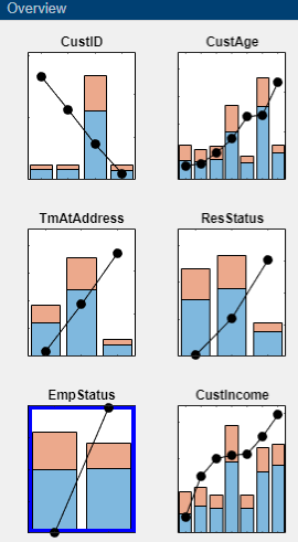
From the main pane, click a bin to enable the Split button for that bin. To deselect a bin, use Ctrl+ click.

On the Binning Explorer toolstrip, click Split to open the Split dialog box for the selected bin.
Note
The Split button is enabled when the selected bin has more than one unique category in it.
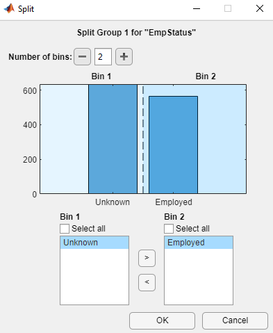
Use the Number of bins control to split the selected bin into multiple bins.
Use the arrow controls on the Split dialog box to control the contents for each of the bins that you are splitting the selected bin into.
Click OK to complete the split operation.
The plot for the selected categorical predictor is updated with the new bin information. The details in the Bin Information and Predictor Information panes are also updated.
Manual Binning to Merge Bins for a Numeric or Categorical Predictor
After you import data or a creditscorecard object
into Binning Explorer, you can split or merge bins for
a predictor.
Click any predictor plot in the Overview pane. The selected predictor plot displays in the main pane.

From the main pane, to merge bins, select two or more bins for merging by using Ctrl + click or Shift + click to multiselect bins to display with blue outlines. To change your bin selection, use Ctrl+ click to deselect a bin.
Note
The Merge button is active only when more than one bin is selected. Only adjacent bins can be merged for numeric or ordinal predictors. Nonadjacent bins can be merged for categorical predictors.
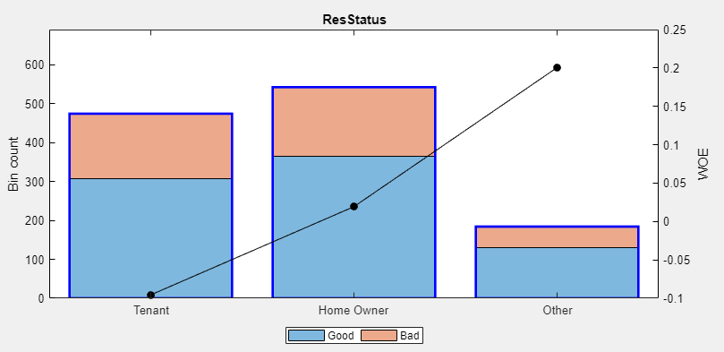
Click Merge to complete the merge operation. The plot for the selected predictor is updated with the new bin information. The details in the Bin Information and Predictor Information panes are also updated.
Change Bin Boundaries for a Single Predictor
After you import data or a creditscorecard object
into Binning Explorer, you can change the bin boundaries
for a single predictor.
Click any numeric predictor plot in the Overview pane. The selected predictor plot displays with a blue outline and the predictor plot displays in the main pane.
From the main pane, click to select a specific bin where you want to change the bin dimensions. The selected bin displays with a blue outline.

On the Binning Explorer toolstrip, the Edges text boxes display values for the edges of the selected bin.

Edit the values in the Edges text boxes to change the selected bin’s dimensions.
Click the main pane to complete the operation. The plot for the predictor is updated with the updated bin’s dimension information. The details in the Bin Information and Predictor Information panes are also updated.
Change Bin Boundaries for Multiple Predictors
After you import data or a creditscorecard object
into Binning Explorer, you can change the algorithm applied
to one or more predictors and you can also redefine the number of
bins.
From the Overview pane, click any predictor plot. The predictor plot displays with a blue outline.

Alternatively, select two or more predictors by using Ctrl + click or Shift + click to multiselect predictors to display with blue outlines.

On the Binning Explorer toolstrip, click Options to open a list of options for the Monotone, Split, Merge, Equal Frequency, and Equal Width algorithms. Click an option to open the associated Algorithm options dialog box. Make your selection from the respective Algorithm Options dialog box and click OK. The selected predictor plots are updated for the change of algorithm and the plots for the selected predictors are updated with the new bin information. The details in the Bin Information and Predictor Information panes are also updated.
Set Options for Display
Binning Explorer has options for displaying predictor plots and plot options and the associated tables displayed in Bin Information.
Plot Options
From the Binning Explorer toolstrip item for Plot Options, select any of the following predictor plot options:
No labels (default)
Bin count
% Bin level
% Data level
% Total count
The selected label is applied to all predictor plots.
Table Options
You can set the table display options for predictor information displayed in Bin Information.
From the Binning Explorer toolstrip item for Table Columns, select any of the following options:
Odds
WOE
InfoValue
Entropy
Gini
Chi2
Members (option is enabled for categorical predictors)
When selected, these options are applied to all predictors for the information displayed in Bin Information.
Export and Save the Binning
Binning Explorer enables you to export and save your credit scorecard binning
definitions to a creditscorecard object. To export a scorecard,
click Export in the Binning Explorer toolstrip. Then, choose
one of the following options:
Click the green check mark.
Click Export Scorecard to open the dropdown menu and click the first option, Export Scorecard.
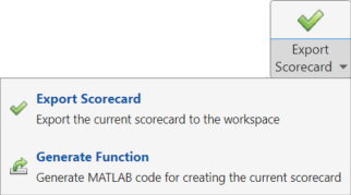
Enter a creditscorecard object name in the Export dialog box.
The creditscorecard object is saved to the MATLAB workspace.
Note
If you export a previously existing creditscorecard
object that was fit (using fitmodel), all fitting
settings in the creditscorecard object are lost. You must
rerun fitmodel on the updated
creditscorecard object.
To reopen a previously saved creditscorecard object, click
Import Data and select the
creditscorecard object from the Step 1
pane of the Import Data window.
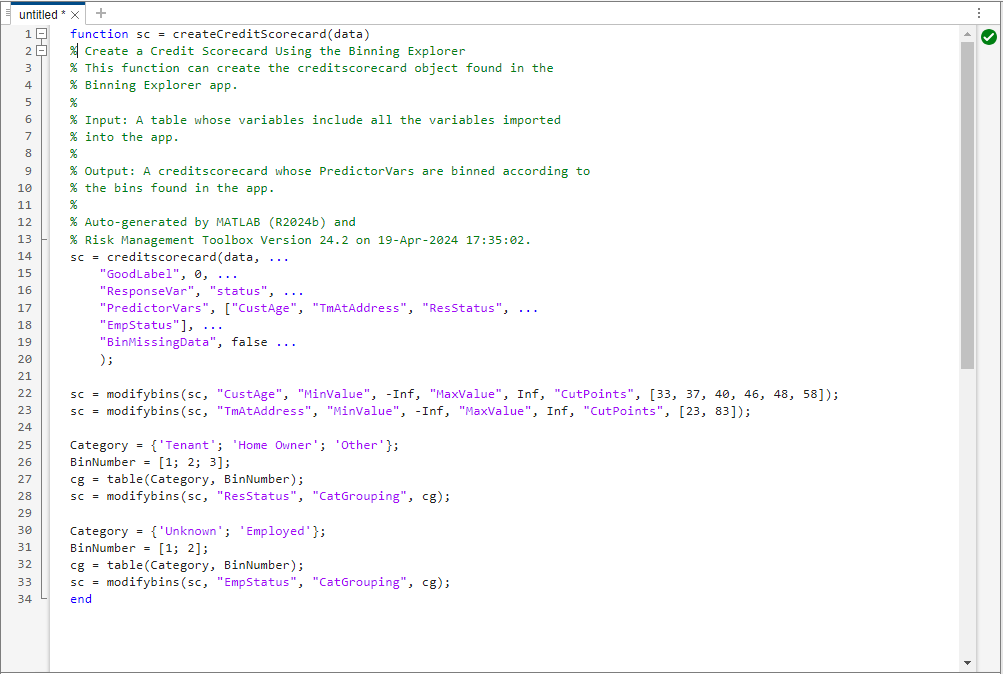
Binning Explorer also enables you to generate a scorecard function that
you can use to create a creditscorecard object. To generate a
scorecard function, follow these steps.
Click Export in the Binning Explorer toolstrip.
Click Export Scorecard to open the dropdown menu.
Click Generate Scorecard Function to open an untitled function in your editor that you can modify and save locally.
Troubleshoot the Binning
This topic shows some of the results when using Binning Explorer with credit scorecards that need troubleshooting. For details on the overall process of creating and developing credit scorecards, see Overview of Binning Explorer and Bin Data to Create Credit Scorecards Using Binning Explorer.
Numeric Predictor Converted to Categorical Predictor Does Not Display Split Data Properly
When you convert a numeric predictor with hundreds of values (for example, continuous data) to categorical data, the resulting data has hundreds of categories. The following example illustrates this scenario.
load CreditCardData
Open the Binning Explorer and select the numeric predictor AMBalance from the Overview pane. From the Binning Explorer toolstrip, change the predictor type to Categorical.
From the Binning Explorer toolstrip and click Split. The Split dialog box displays as follows:
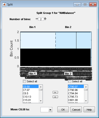
The predictor has too many categories to display properly.
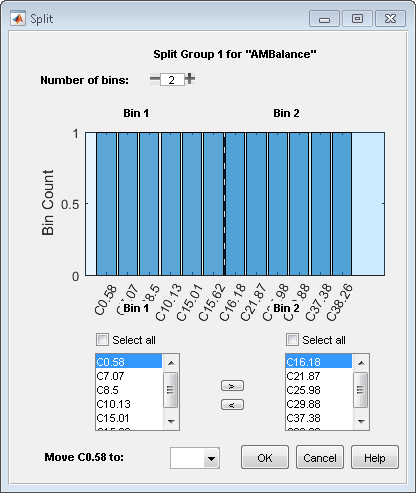
Solution: If you have a categorical predictor with a large
number of categories, use the Algorithm Options to change
the binning algorithm for that predictor to Equal
Frequency, with the Number of bins set to
100 (or another smaller value). The Split dialog box then
displays properly.
Predictor Plot Appears Distorted
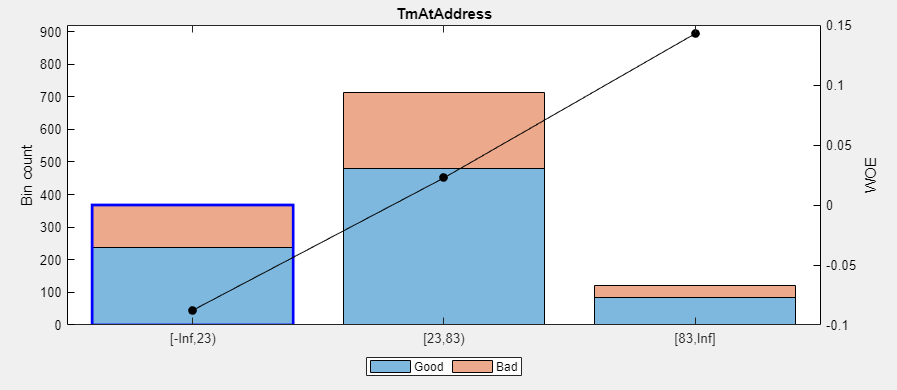
When using the Binning Explorer, if you import data that has not been previously binned and you select No Binning from the Import Data window, the resulting plots might be distorted. For example, if you load the following data set into the MATLAB workspace and use Binning Explorer to import the data using No Binning, the following plot displays for the TmAtAddress predictor.
load CreditCardData

Solution: When you import data that has not been previously binned, select Monotone from the Import Data window instead. The following plot displays for the TmAtAddress predictor.
See Also
Apps
Classes
Topics
- Bin Data to Create Credit Scorecards Using Binning Explorer
- Case Study for Credit Scorecard Analysis
- Credit Scorecard Modeling with Missing Values
- Overview of Binning Explorer
- Credit Scorecard Modeling Workflow