Case Study for Credit Scorecard Analysis
This example shows how to create a creditscorecard object, bin data, display, and plot binned data information. This example also shows how to fit a logistic regression model, obtain a score for the scorecard model, and determine the probabilities of default and validate the credit scorecard model using three different metrics.
Step 1. Create a creditscorecard object.
Use the CreditCardData.mat file to load the data (using a dataset from Refaat 2011). If your data contains many predictors, you can first use screenpredictors (Risk Management Toolbox) to pare down a potentially large set of predictors to a subset that is most predictive of the credit scorecard response variable. You can then use this subset of predictors when creating the creditscorecard object. In addition, you can use Threshold Predictors (Risk Management Toolbox) to interactively set credit scorecard predictor thresholds using the output from screenpredictors (Risk Management Toolbox).
When creating a creditscorecard object, by default, 'ResponseVar' is set to the last column in the data ('status' in this example) and the 'GoodLabel' to the response value with the highest count (0 in this example). The syntax for creditscorecard indicates that 'CustID' is the 'IDVar' to remove from the list of predictors. Also, while not demonstrated in this example, when creating a creditscorecard object using creditscorecard, you can use the optional name-value pair argument 'WeightsVar' to specify observation (sample) weights or 'BinMissingData' to bin missing data.
load CreditCardData
head(data)
CustID CustAge TmAtAddress ResStatus EmpStatus CustIncome TmWBank OtherCC AMBalance UtilRate status
______ _______ ___________ __________ _________ __________ _______ _______ _________ ________ ______
1 53 62 Tenant Unknown 50000 55 Yes 1055.9 0.22 0
2 61 22 Home Owner Employed 52000 25 Yes 1161.6 0.24 0
3 47 30 Tenant Employed 37000 61 No 877.23 0.29 0
4 50 75 Home Owner Employed 53000 20 Yes 157.37 0.08 0
5 68 56 Home Owner Employed 53000 14 Yes 561.84 0.11 0
6 65 13 Home Owner Employed 48000 59 Yes 968.18 0.15 0
7 34 32 Home Owner Unknown 32000 26 Yes 717.82 0.02 1
8 50 57 Other Employed 51000 33 No 3041.2 0.13 0
The variables in CreditCardData are customer ID, customer age, time at current address, residential status, employment status, customer income, time with bank, other credit card, average monthly balance, utilization rate, and the default status (response).
sc = creditscorecard(data,'IDVar','CustID')
sc =
  creditscorecard with properties:

                GoodLabel: 0
              ResponseVar: 'status'
               WeightsVar: ''
                 VarNames: {'CustID'  'CustAge'  'TmAtAddress'  'ResStatus'  'EmpStatus'  'CustIncome'  'TmWBank'  'OtherCC'  'AMBalance'  'UtilRate'  'status'}
        NumericPredictors: {'CustAge'  'TmAtAddress'  'CustIncome'  'TmWBank'  'AMBalance'  'UtilRate'}
    CategoricalPredictors: {'ResStatus'  'EmpStatus'  'OtherCC'}
           BinMissingData: 0
                    IDVar: 'CustID'
            PredictorVars: {'CustAge'  'TmAtAddress'  'ResStatus'  'EmpStatus'  'CustIncome'  'TmWBank'  'OtherCC'  'AMBalance'  'UtilRate'}
                     Data: [1200×11 table]
Perform some initial data exploration. Inquire about predictor statistics for the categorical variable 'ResStatus' and plot the bin information for 'ResStatus'.
bininfo(sc,'ResStatus')ans=4×6 table
Bin Good Bad Odds WOE InfoValue
______________ ____ ___ ______ _________ _________
{'Home Owner'} 365 177 2.0621 0.019329 0.0001682
{'Tenant' } 307 167 1.8383 -0.095564 0.0036638
{'Other' } 131 53 2.4717 0.20049 0.0059418
{'Totals' } 803 397 2.0227 NaN 0.0097738
plotbins(sc,'ResStatus')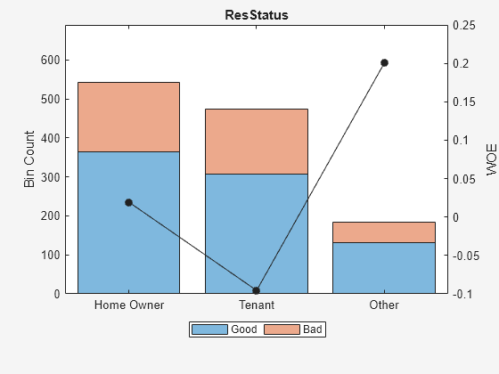
This bin information contains the frequencies of “Good” and “Bad,” and bin statistics. Avoid having bins with frequencies of zero because they lead to infinite or undefined (NaN) statistics. Use the modifybins or autobinning functions to bin the data accordingly.
For numeric data, a common first step is "fine classing." This means binning the data into several bins, defined with a regular grid. To illustrate this point, use the predictor 'CustIncome'.
cp = 20000:5000:60000;

sc = modifybins(sc,'CustIncome','CutPoints',cp);

bininfo(sc,'CustIncome')
ans=11×6 table
           Bin           Good    Bad     Odds         WOE       InfoValue
    _________________    ____    ___    _______    _________    __________

    {'[-Inf,20000)' }      3       5        0.6      -1.2152      0.010765
    {'[20000,25000)'}     23      16     1.4375     -0.34151     0.0039819
    {'[25000,30000)'}     38      47    0.80851     -0.91698      0.065166
    {'[30000,35000)'}    131      75     1.7467     -0.14671      0.003782
    {'[35000,40000)'}    193      98     1.9694    -0.026696    0.00017359
    {'[40000,45000)'}    173      76     2.2763      0.11814     0.0028361
    {'[45000,50000)'}    131      47     2.7872      0.32063      0.014348
    {'[50000,55000)'}     82      24     3.4167      0.52425      0.021842
    {'[55000,60000)'}     21       8      2.625      0.26066     0.0015642
    {'[60000,Inf]'  }      8       1          8        1.375      0.010235
    {'Totals'       }    803     397     2.0227          NaN       0.13469
plotbins(sc,'CustIncome')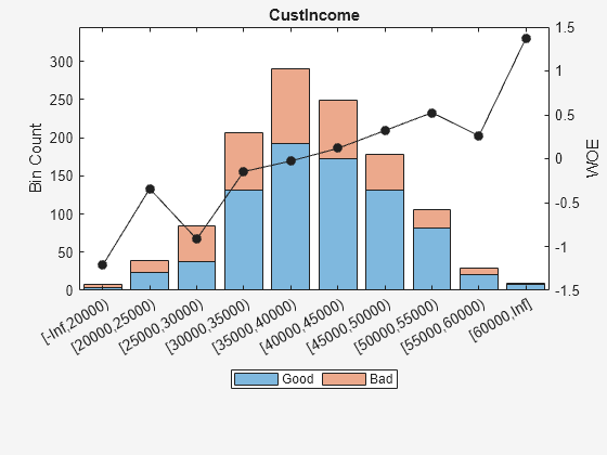
Step 2a. Automatically bin the data.
Use the autobinning function to perform automatic binning for every predictor variable, using the default 'Monotone' algorithm with default algorithm options.
sc = autobinning(sc);
After the automatic binning step, every predictor bin must be reviewed using the bininfo and plotbins functions and fine-tuned. A monotonic, ideally linear trend in the Weight of Evidence (WOE) is desirable for credit scorecards because this translates into linear points for a given predictor. The WOE trends can be visualized using plotbins.
Predictor = 'ResStatus';
plotbins(sc,Predictor)
'ResStatus';
plotbins(sc,Predictor)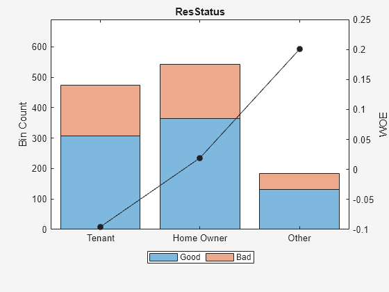
Unlike the initial plot of 'ResStatus' when the scorecard was created, the new plot for 'ResStatus' shows an increasing WOE trend. This is because the autobinning function, by default, sorts the order of the categories by increasing odds.
These plots show that the 'Monotone' algorithm does a good job finding monotone WOE trends for this dataset. To complete the binning process, it is necessary to make only a few manual adjustments for some predictors using the modifybins function.
Step 2b. Fine-tune the bins using manual binning.
Common steps to manually modify bins are:
Use the
bininfofunction with two output arguments where the second argument contains binning rules.Manually modify the binning rules using the second output argument from
bininfo.Set the updated binning rules with
modifybinsand then useplotbinsorbininfoto review the updated bins.
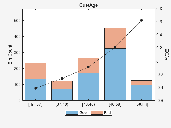
For example, based on the plot for 'CustAge' in Step 2a, bins number 1 and 2 have similar WOE's as do bins number 5 and 6. To merge these bins using the steps outlined above:
Predictor = 'CustAge';
[bi,cp] = bininfo(sc,Predictor)
'CustAge';
[bi,cp] = bininfo(sc,Predictor)bi=8×6 table
Bin Good Bad Odds WOE InfoValue
_____________ ____ ___ ______ _________ _________
{'[-Inf,33)'} 70 53 1.3208 -0.42622 0.019746
{'[33,37)' } 64 47 1.3617 -0.39568 0.015308
{'[37,40)' } 73 47 1.5532 -0.26411 0.0072573
{'[40,46)' } 174 94 1.8511 -0.088658 0.001781
{'[46,48)' } 61 25 2.44 0.18758 0.0024372
{'[48,58)' } 263 105 2.5048 0.21378 0.013476
{'[58,Inf]' } 98 26 3.7692 0.62245 0.0352
{'Totals' } 803 397 2.0227 NaN 0.095205
cp = 6×1

    33
    37
    40
    46
    48
    58
cp([1 5]) = []; % To merge bins 1 and 2, and bins 5 and 6
sc = modifybins(sc,'CustAge','CutPoints',cp);
plotbins(sc,'CustAge')
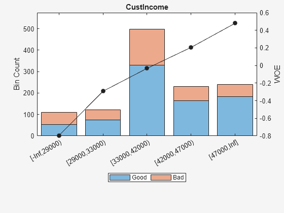
For 'CustIncome', based on the plot above, it is best to merge bins 3, 4 and 5 because they have similar WOE's. To merge these bins:
Predictor = 'CustIncome';
[bi,cp] = bininfo(sc,Predictor)
'CustIncome';
[bi,cp] = bininfo(sc,Predictor)bi=8×6 table
Bin Good Bad Odds WOE InfoValue
_________________ ____ ___ _______ _________ __________
{'[-Inf,29000)' } 53 58 0.91379 -0.79457 0.06364
{'[29000,33000)'} 74 49 1.5102 -0.29217 0.0091366
{'[33000,35000)'} 68 36 1.8889 -0.06843 0.00041042
{'[35000,40000)'} 193 98 1.9694 -0.026696 0.00017359
{'[40000,42000)'} 68 34 2 -0.011271 1.0819e-05
{'[42000,47000)'} 164 66 2.4848 0.20579 0.0078175
{'[47000,Inf]' } 183 56 3.2679 0.47972 0.041657
{'Totals' } 803 397 2.0227 NaN 0.12285
cp = 6×1

       29000
       33000
       35000
       40000
       42000
       47000
cp([3 4]) = []; % To merge bins 3, 4, and 5
sc = modifybins(sc,'CustIncome','CutPoints',cp);
plotbins(sc,'CustIncome')
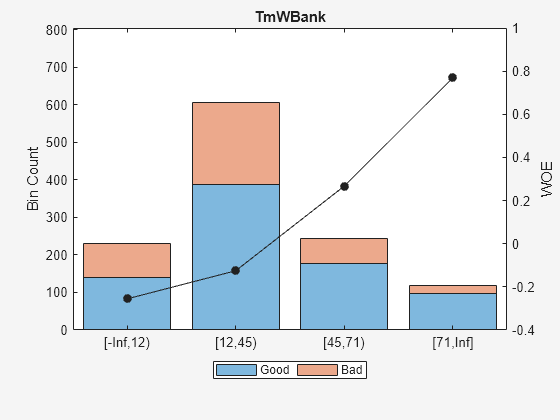
For 'TmWBank', based on the plot above, it is best to merge bins 2 and 3 because they have similar WOE's. To merge these bins:
Predictor = 'TmWBank';
[bi,cp] = bininfo(sc,Predictor)
'TmWBank';
[bi,cp] = bininfo(sc,Predictor)bi=6×6 table
Bin Good Bad Odds WOE InfoValue
_____________ ____ ___ ______ ________ _________
{'[-Inf,12)'} 141 90 1.5667 -0.25547 0.013057
{'[12,23)' } 165 93 1.7742 -0.13107 0.0037719
{'[23,45)' } 224 125 1.792 -0.12109 0.0043479
{'[45,71)' } 177 67 2.6418 0.26704 0.013795
{'[71,Inf]' } 96 22 4.3636 0.76889 0.049313
{'Totals' } 803 397 2.0227 NaN 0.084284
cp = 4×1

    12
    23
    45
    71
cp(2) = []; % To merge bins 2 and 3
sc = modifybins(sc,'TmWBank','CutPoints',cp);
plotbins(sc,'TmWBank')
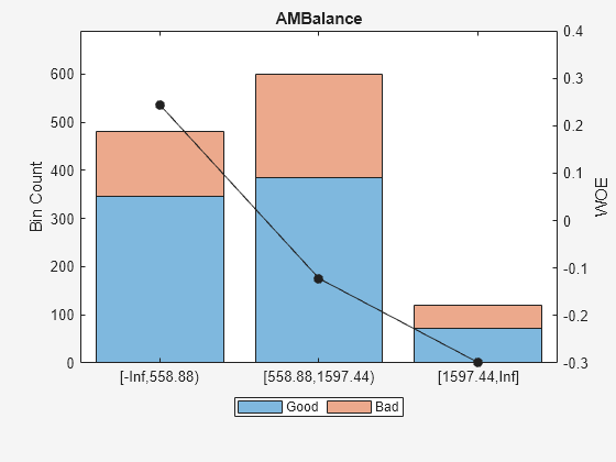
For 'AMBalance', based on the plot above, it is best to merge bins 2 and 3 because they have similar WOE's. To merge these bins:
Predictor = 'AMBalance';
[bi,cp] = bininfo(sc,Predictor)
'AMBalance';
[bi,cp] = bininfo(sc,Predictor)bi=5×6 table
Bin Good Bad Odds WOE InfoValue
_____________________ ____ ___ ______ ________ _________
{'[-Inf,558.88)' } 346 134 2.5821 0.24418 0.022795
{'[558.88,1254.28)' } 309 171 1.807 -0.11274 0.0051774
{'[1254.28,1597.44)'} 76 44 1.7273 -0.15787 0.0025554
{'[1597.44,Inf]' } 72 48 1.5 -0.29895 0.0093402
{'Totals' } 803 397 2.0227 NaN 0.039868
cp = 3×1
103 ×

    0.5589
    1.2543
    1.5974
cp(2) = []; % To merge bins 2 and 3
sc = modifybins(sc,'AMBalance','CutPoints',cp);
plotbins(sc,'AMBalance')
Now that the binning fine-tuning is completed, the bins for all predictors have close-to-linear WOE trends.
Step 3. Fit a logistic regression model.
The fitmodel function fits a logistic regression model to the WOE data. fitmodel internally bins the training data, transforms it into WOE values, maps the response variable so that 'Good' is 1, and fits a linear logistic regression model. By default, fitmodel uses a stepwise procedure to determine which predictors should be in the model.
sc = fitmodel(sc);
1. Adding CustIncome, Deviance = 1490.8954, Chi2Stat = 32.545914, PValue = 1.1640961e-08
2. Adding TmWBank, Deviance = 1467.3249, Chi2Stat = 23.570535, PValue = 1.2041739e-06
3. Adding AMBalance, Deviance = 1455.858, Chi2Stat = 11.466846, PValue = 0.00070848829
4. Adding EmpStatus, Deviance = 1447.6148, Chi2Stat = 8.2432677, PValue = 0.0040903428
5. Adding CustAge, Deviance = 1442.06, Chi2Stat = 5.5547849, PValue = 0.018430237
6. Adding ResStatus, Deviance = 1437.9435, Chi2Stat = 4.1164321, PValue = 0.042468555
7. Adding OtherCC, Deviance = 1433.7372, Chi2Stat = 4.2063597, PValue = 0.040272676

Generalized linear regression model:
    logit(status) ~ 1 + CustAge + ResStatus + EmpStatus + CustIncome + TmWBank + OtherCC + AMBalance
    Distribution = Binomial

Estimated Coefficients:
                   Estimate      SE       tStat       pValue
                   ________    _______    ______    __________

    (Intercept)     0.7024       0.064    10.975    5.0407e-28
    CustAge        0.61562     0.24783    2.4841      0.012988
    ResStatus       1.3776     0.65266    2.1107      0.034799
    EmpStatus      0.88592     0.29296     3.024     0.0024946
    CustIncome     0.69836     0.21715     3.216     0.0013001
    TmWBank          1.106     0.23266    4.7538    1.9958e-06
    OtherCC         1.0933     0.52911    2.0662      0.038806
    AMBalance       1.0437     0.32292    3.2322     0.0012285


1200 observations, 1192 error degrees of freedom
Dispersion: 1
Chi^2-statistic vs. constant model: 89.7, p-value = 1.42e-16
Step 4. Review and format scorecard points.
After fitting the logistic model, by default the points are unscaled and come directly from the combination of WOE values and model coefficients. The displaypoints function summarizes the scorecard points.
p1 = displaypoints(sc);
disp(p1)
      Predictors              Bin              Points
    ______________    ____________________    _________

    {'CustAge'   }    {'[-Inf,37)'       }     -0.15314
    {'CustAge'   }    {'[37,40)'         }    -0.062247
    {'CustAge'   }    {'[40,46)'         }     0.045763
    {'CustAge'   }    {'[46,58)'         }      0.22888
    {'CustAge'   }    {'[58,Inf]'        }      0.48354
    {'CustAge'   }    {'<missing>'       }          NaN
    {'ResStatus' }    {'Tenant'          }    -0.031302
    {'ResStatus' }    {'Home Owner'      }      0.12697
    {'ResStatus' }    {'Other'           }      0.37652
    {'ResStatus' }    {'<missing>'       }          NaN
    {'EmpStatus' }    {'Unknown'         }    -0.076369
    {'EmpStatus' }    {'Employed'        }      0.31456
    {'EmpStatus' }    {'<missing>'       }          NaN
    {'CustIncome'}    {'[-Inf,29000)'    }     -0.45455
    {'CustIncome'}    {'[29000,33000)'   }      -0.1037
    {'CustIncome'}    {'[33000,42000)'   }     0.077768
    {'CustIncome'}    {'[42000,47000)'   }      0.24406
    {'CustIncome'}    {'[47000,Inf]'     }      0.43536
    {'CustIncome'}    {'<missing>'       }          NaN
    {'TmWBank'   }    {'[-Inf,12)'       }     -0.18221
    {'TmWBank'   }    {'[12,45)'         }    -0.038279
    {'TmWBank'   }    {'[45,71)'         }      0.39569
    {'TmWBank'   }    {'[71,Inf]'        }      0.95074
    {'TmWBank'   }    {'<missing>'       }          NaN
    {'OtherCC'   }    {'No'              }       -0.193
    {'OtherCC'   }    {'Yes'             }      0.15868
    {'OtherCC'   }    {'<missing>'       }          NaN
    {'AMBalance' }    {'[-Inf,558.88)'   }       0.3552
    {'AMBalance' }    {'[558.88,1597.44)'}    -0.026797
    {'AMBalance' }    {'[1597.44,Inf]'   }     -0.21168
    {'AMBalance' }    {'<missing>'       }          NaN
This is a good time to modify the bin labels, if this is something of interest for cosmetic reasons. To do so, use modifybins to change the bin labels.
sc = modifybins(sc,'CustAge','BinLabels',...
{'Up to 36' '37 to 39' '40 to 45' '46 to 57' '58 and up'});

sc = modifybins(sc,'CustIncome','BinLabels',...
{'Up to 28999' '29000 to 32999' '33000 to 41999' '42000 to 46999' '47000 and up'});

sc = modifybins(sc,'TmWBank','BinLabels',...
{'Up to 11' '12 to 44' '45 to 70' '71 and up'});

sc = modifybins(sc,'AMBalance','BinLabels',...
{'Up to 558.87' '558.88 to 1597.43' '1597.44 and up'});

p1 = displaypoints(sc);
disp(p1)
      Predictors               Bin              Points
    ______________    _____________________    _________

    {'CustAge'   }    {'Up to 36'         }     -0.15314
    {'CustAge'   }    {'37 to 39'         }    -0.062247
    {'CustAge'   }    {'40 to 45'         }     0.045763
    {'CustAge'   }    {'46 to 57'         }      0.22888
    {'CustAge'   }    {'58 and up'        }      0.48354
    {'CustAge'   }    {'<missing>'        }          NaN
    {'ResStatus' }    {'Tenant'           }    -0.031302
    {'ResStatus' }    {'Home Owner'       }      0.12697
    {'ResStatus' }    {'Other'            }      0.37652
    {'ResStatus' }    {'<missing>'        }          NaN
    {'EmpStatus' }    {'Unknown'          }    -0.076369
    {'EmpStatus' }    {'Employed'         }      0.31456
    {'EmpStatus' }    {'<missing>'        }          NaN
    {'CustIncome'}    {'Up to 28999'      }     -0.45455
    {'CustIncome'}    {'29000 to 32999'   }      -0.1037
    {'CustIncome'}    {'33000 to 41999'   }     0.077768
    {'CustIncome'}    {'42000 to 46999'   }      0.24406
    {'CustIncome'}    {'47000 and up'     }      0.43536
    {'CustIncome'}    {'<missing>'        }          NaN
    {'TmWBank'   }    {'Up to 11'         }     -0.18221
    {'TmWBank'   }    {'12 to 44'         }    -0.038279
    {'TmWBank'   }    {'45 to 70'         }      0.39569
    {'TmWBank'   }    {'71 and up'        }      0.95074
    {'TmWBank'   }    {'<missing>'        }          NaN
    {'OtherCC'   }    {'No'               }       -0.193
    {'OtherCC'   }    {'Yes'              }      0.15868
    {'OtherCC'   }    {'<missing>'        }          NaN
    {'AMBalance' }    {'Up to 558.87'     }       0.3552
    {'AMBalance' }    {'558.88 to 1597.43'}    -0.026797
    {'AMBalance' }    {'1597.44 and up'   }     -0.21168
    {'AMBalance' }    {'<missing>'        }          NaN
Points are usually scaled and also often rounded. To do this, use the formatpoints function. For example, you can set a target level of points corresponding to a target odds level and also set the required points-to-double-the-odds (PDO).
TargetPoints = 500;
TargetOdds = 2;
PDO = 50; % Points to double the odds

sc = formatpoints(sc,'PointsOddsAndPDO',[TargetPoints TargetOdds PDO]);
p2 = displaypoints(sc);
disp(p2)
      Predictors               Bin             Points
    ______________    _____________________    ______

    {'CustAge'   }    {'Up to 36'         }    53.239
    {'CustAge'   }    {'37 to 39'         }    59.796
    {'CustAge'   }    {'40 to 45'         }    67.587
    {'CustAge'   }    {'46 to 57'         }    80.796
    {'CustAge'   }    {'58 and up'        }    99.166
    {'CustAge'   }    {'<missing>'        }       NaN
    {'ResStatus' }    {'Tenant'           }    62.028
    {'ResStatus' }    {'Home Owner'       }    73.445
    {'ResStatus' }    {'Other'            }    91.446
    {'ResStatus' }    {'<missing>'        }       NaN
    {'EmpStatus' }    {'Unknown'          }    58.777
    {'EmpStatus' }    {'Employed'         }    86.976
    {'EmpStatus' }    {'<missing>'        }       NaN
    {'CustIncome'}    {'Up to 28999'      }    31.497
    {'CustIncome'}    {'29000 to 32999'   }    56.805
    {'CustIncome'}    {'33000 to 41999'   }    69.896
    {'CustIncome'}    {'42000 to 46999'   }    81.891
    {'CustIncome'}    {'47000 and up'     }     95.69
    {'CustIncome'}    {'<missing>'        }       NaN
    {'TmWBank'   }    {'Up to 11'         }    51.142
    {'TmWBank'   }    {'12 to 44'         }    61.524
    {'TmWBank'   }    {'45 to 70'         }    92.829
    {'TmWBank'   }    {'71 and up'        }    132.87
    {'TmWBank'   }    {'<missing>'        }       NaN
    {'OtherCC'   }    {'No'               }    50.364
    {'OtherCC'   }    {'Yes'              }    75.732
    {'OtherCC'   }    {'<missing>'        }       NaN
    {'AMBalance' }    {'Up to 558.87'     }    89.908
    {'AMBalance' }    {'558.88 to 1597.43'}    62.353
    {'AMBalance' }    {'1597.44 and up'   }    49.016
    {'AMBalance' }    {'<missing>'        }       NaN
Step 5. Score the data.
The score function computes the scores for the training data. An optional data input can also be passed to score, for example, validation data. The points per predictor for each customer are provided as an optional output.
[Scores,Points] = score(sc);
disp(Scores(1:10))
  528.2044
  554.8861
  505.2406
  564.0717
  554.8861
  586.1904
  441.8755
  515.8125
  524.4553
  508.3169
disp(Points(1:10,:))
    CustAge    ResStatus    EmpStatus    CustIncome    TmWBank    OtherCC    AMBalance
    _______    _________    _________    __________    _______    _______    _________

    80.796      62.028       58.777         95.69      92.829     75.732      62.353
    99.166      73.445       86.976         95.69      61.524     75.732      62.353
    80.796      62.028       86.976        69.896      92.829     50.364      62.353
    80.796      73.445       86.976         95.69      61.524     75.732      89.908
    99.166      73.445       86.976         95.69      61.524     75.732      62.353
    99.166      73.445       86.976         95.69      92.829     75.732      62.353
    53.239      73.445       58.777        56.805      61.524     75.732      62.353
    80.796      91.446       86.976         95.69      61.524     50.364      49.016
    80.796      62.028       58.777         95.69      61.524     75.732      89.908
    80.796      73.445       58.777         95.69      61.524     75.732      62.353
Step 6. Calculate the probability of default.
To calculate the probability of default, use the probdefault function.
pd = probdefault(sc);
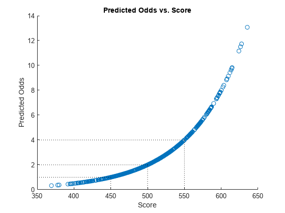
Define the probability of being “Good” and plot the predicted odds versus the formatted scores. Visually analyze that the target points and target odds match and that the points-to-double-the-odds (PDO) relationship holds.
ProbGood = 1-pd;
PredictedOdds = ProbGood./pd;

figure
scatter(Scores,PredictedOdds)
title('Predicted Odds vs. Score')
xlabel('Score')
ylabel('Predicted Odds')

hold on

xLimits = xlim;
yLimits = ylim;

% Target points and odds
plot([TargetPoints TargetPoints],[yLimits(1) TargetOdds],'k:')
plot([xLimits(1) TargetPoints],[TargetOdds TargetOdds],'k:')

% Target points plus PDO
plot([TargetPoints+PDO TargetPoints+PDO],[yLimits(1) 2*TargetOdds],'k:')
plot([xLimits(1) TargetPoints+PDO],[2*TargetOdds 2*TargetOdds],'k:')

% Target points minus PDO
plot([TargetPoints-PDO TargetPoints-PDO],[yLimits(1) TargetOdds/2],'k:')
plot([xLimits(1) TargetPoints-PDO],[TargetOdds/2 TargetOdds/2],'k:')

hold off
Step 7. Validate the credit scorecard model using the CAP, ROC, and Kolmogorov-Smirnov statistic
The creditscorecard class supports three validation methods, the Cumulative Accuracy Profile (CAP), the Receiver Operating Characteristic (ROC), and the Kolmogorov-Smirnov (KS) statistic. For more information on CAP, ROC, and KS, see Cumulative Accuracy Profile (CAP), Receiver Operating Characteristic (ROC), and Kolmogorov-Smirnov statistic (KS).
[Stats,T] = validatemodel(sc,'Plot',{'CAP','ROC','KS'});
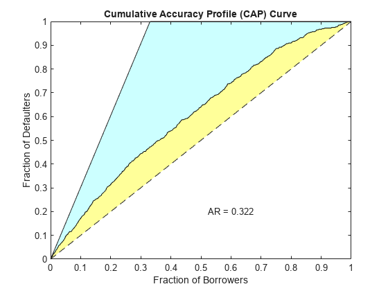
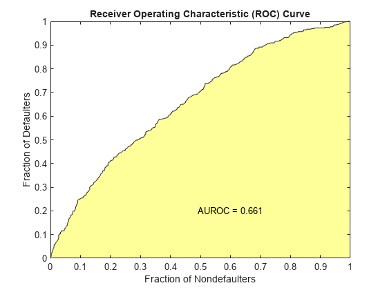
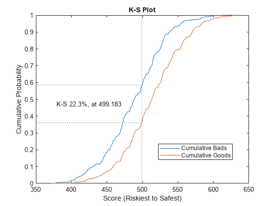
disp(Stats)
            Measure              Value
    ________________________    _______

    {'Accuracy Ratio'      }    0.32225
    {'Area under ROC curve'}    0.66113
    {'KS statistic'        }    0.22324
    {'KS score'            }     499.18
disp(T(1:15,:))
    Scores    ProbDefault    TrueBads    FalseBads    TrueGoods    FalseGoods    Sensitivity    FalseAlarm      PctObs
    ______    ___________    ________    _________    _________    __________    ___________    __________    __________

     369.4       0.7535          0           1           802          397                 0     0.0012453     0.00083333
    377.86      0.73107          1           1           802          396         0.0025189     0.0012453      0.0016667
    379.78       0.7258          2           1           802          395         0.0050378     0.0012453         0.0025
    391.81      0.69139          3           1           802          394         0.0075567     0.0012453      0.0033333
    394.77      0.68259          3           2           801          394         0.0075567     0.0024907      0.0041667
    395.78      0.67954          4           2           801          393          0.010076     0.0024907          0.005
    396.95      0.67598          5           2           801          392          0.012594     0.0024907      0.0058333
    398.37      0.67167          6           2           801          391          0.015113     0.0024907      0.0066667
    401.26      0.66276          7           2           801          390          0.017632     0.0024907         0.0075
    403.23      0.65664          8           2           801          389          0.020151     0.0024907      0.0083333
    405.09      0.65081          8           3           800          389          0.020151      0.003736      0.0091667
    405.15      0.65062         11           5           798          386          0.027708     0.0062267       0.013333
    405.37      0.64991         11           6           797          386          0.027708      0.007472       0.014167
    406.18      0.64735         12           6           797          385          0.030227      0.007472          0.015
    407.14      0.64433         13           6           797          384          0.032746      0.007472       0.015833
Step 8. Validate at Decile Level
In step 7, the validatemodel function uses the default 'AnalysisLevel' at the individual score level. Now consider using the validatemodel function with 'decile' level validation statistics.
[Stats,T] = validatemodel(sc,'AnalysisLevel','deciles');
disp(Stats)
            Measure              Value
    ________________________    _______

    {'Accuracy Ratio'      }    0.31659
    {'Area under ROC curve'}     0.6583
    {'KS statistic'        }    0.21543
    {'KS score'            }     482.52
disp(T)
    Scores    ProbDefault    TrueBads    FalseBads    TrueGoods    FalseGoods    Sensitivity    FalseAlarm    PctObs
    ______    ___________    ________    _________    _________    __________    ___________    __________    _______

    447.51      0.57922         68           52          751          329          0.17128       0.064757         0.1
    469.34       0.4678        125          115          688          272          0.31486        0.14321         0.2
    482.52      0.41453        176          183          620          221          0.44332         0.2279     0.29917
     496.7      0.37202        214          265          538          183          0.53904        0.33001     0.39917
    504.49      0.33294        254          345          458          143           0.6398        0.42964     0.49917
    515.51      0.29986        294          426          377          103          0.74055        0.53051         0.6
    528.08       0.2691        330          510          293           67          0.83123        0.63512         0.7
    541.38      0.23827        361          599          204           36          0.90932        0.74595         0.8
    563.16      0.19765        384          696          107           13          0.96725        0.86675         0.9
    635.41      0.13789        397          803            0            0                1              1           1
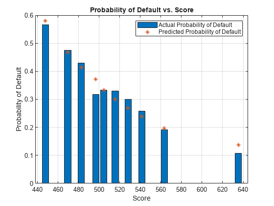
You can use the validation statistics to display the actual and predicted probabilities of default at the decile level.
% The TrueBads and FalseBads columns contain cumulative data
bads = diff([0;T.TrueBads]);
goods = diff([0;T.FalseBads]);
obsPD = bads./(bads+goods);
predPD = T.ProbDefault;
bar(T.Scores,obsPD)
hold on
scatter(T.Scores,predPD,'*')
xlabel('Score')
ylabel('Probability of Default')
title('Probability of Default vs. Score')
grid
legend('Actual Probability of Default', 'Predicted Probability of Default')
hold off
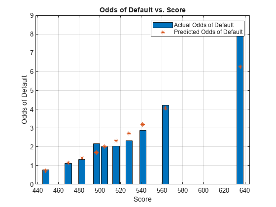
Similarly, you can consider the actual and predicted odds of default.
obsOdds = (1-obsPD)./obsPD;
predOdds = (1-predPD)./predPD;
bar(T.Scores,obsOdds)
hold on
scatter(T.Scores,predOdds,'*')
xlabel('Score')
ylabel('Odds of Default')
title('Odds of Default vs. Score')
grid
legend('Actual Odds of Default', 'Predicted Odds of Default')
hold off
Finally, compute the Hosmer-Lemeshow statistic. Recall that the null hypothesis of the Hosmer-Lemeshow test is that the actual (observed) and predicted (expected) probability of default is the same. Thus, a small p-value that rejects the null hypothesis is an indicator of a poor model fit.
N = bads+goods;
obsBads = bads;
expBads = predPD.*N;
HLStatistic = sum((obsBads-expBads).^2./(N.*predPD.*(1-predPD)));
% 8 degrees of freedom = 10 (deciles) - 2
pHL = chi2cdf(HLStatistic,8,'upper')
pHL =
0.8503
See Also
creditscorecard | autobinning | bininfo | predictorinfo | modifypredictor | modifybins | bindata | plotbins | fitmodel | displaypoints | formatpoints | score | setmodel | probdefault | validatemodel | compact
Topics
- Troubleshooting Credit Scorecard Results
- Credit Rating by Bagging Decision Trees
- About Credit Scorecards
- Credit Scorecard Modeling Workflow
- Credit Scorecard Modeling Using Observation Weights
- Monotone Adjacent Pooling Algorithm (MAPA)