Create Weighted LGD Model

Open Live Script

This example shows how to use the fitLGDModel function to create an LGD model using weighted portfolio data. There are many reasons to create a weighted LGD model. For example, consider the scenarios where you want to weight newer data more heavily than older data, or weight certain data points more heavily because they are more relevant to the purposes of a business. In this example, you use LGD portfolio data and assign more weight to investment loans than residential loans.

Load Data

First, load the LGD portfolio data which consists of residential and investment type loans.

load LGDData.mat
disp(head(data))

      LTV        Age         Type           LGD   
    _______    _______    ___________    _________

    0.89101    0.39716    residential     0.032659
    0.70176     2.0939    residential      0.43564
    0.72078     2.7948    residential    0.0064766
    0.37013      1.237    residential     0.007947
    0.36492     2.5818    residential            0
      0.796     1.5957    residential      0.14572
    0.60203     1.1599    residential     0.025688
    0.92005    0.50253    investment      0.063182

Create Weights Variable

In this example, assume that the residential loans in the portfolio principally originate as investment loans or that investment loans tend to be larger. Construct a weights variable and assign weights of 1 and 0.1 for investment and residential loans, respectively.

weightedData = data;
weightedData.WeightsByType = ones(height(weightedData),1);
weightedData.WeightsByType(weightedData.Type=='residential') = 0.1;
disp(head(weightedData))

      LTV        Age         Type           LGD       WeightsByType
    _______    _______    ___________    _________    _____________

    0.89101    0.39716    residential     0.032659         0.1     
    0.70176     2.0939    residential      0.43564         0.1     
    0.72078     2.7948    residential    0.0064766         0.1     
    0.37013      1.237    residential     0.007947         0.1     
    0.36492     2.5818    residential            0         0.1     
      0.796     1.5957    residential      0.14572         0.1     
    0.60203     1.1599    residential     0.025688         0.1     
    0.92005    0.50253    investment      0.063182           1

Create LGD Model

Specify a regression LGD model, and then use fitLGDModel to fit a weighted model with the WeightsVar name-value argument.

LGDmodel = fitLGDModel(weightedData,"regression",PredictorVars={'LTV','Age','Type'},ResponseVar="LGD",WeightsVar="WeightsByType");
disp(LGDmodel)

  Regression with properties:

    ResponseTransform: "logit"
    BoundaryTolerance: 1.0000e-05
              ModelID: "Regression"
          Description: ""
      UnderlyingModel: [1x1 classreg.regr.CompactLinearModel]
        PredictorVars: ["LTV"    "Age"    "Type"]
          ResponseVar: "LGD"
           WeightsVar: "WeightsByType"

Display the underlying model.

disp(LGDmodel.UnderlyingModel)

Compact linear regression model:
    LGD_logit ~ 1 + LTV + Age + Type

Estimated Coefficients:
                       Estimate       SE        tStat       pValue   
                       ________    ________    _______    ___________

    (Intercept)         -5.029      0.28058    -17.924     8.6279e-69
    LTV                 3.3166      0.30562     10.852     5.2479e-27
    Age                -1.6089     0.068496    -23.489    2.2385e-113
    Type_investment     1.3639      0.15856     8.6016     1.1698e-17


Number of observations: 3487, Error degrees of freedom: 3483
Root Mean Squared Error: 2.2
R-squared: 0.21,  Adjusted R-Squared: 0.21
F-statistic vs. constant model: 309, p-value = 4.17e-178

Validate Model

Use the modelDiscrimination function to view the area under ROC (AUROC) metric for different segments of the validation data. When ShowDetails is true, you have three extra columns in the DiscMeasure output: Segment, SegmentCount, and WeightedCount. Segment shows the segmentation variable value corresponding to the given row. SegmentCount gives the number of data points contained by the given segment, while WeightedCount shows the sum of the weights associated with the segment data. The default weight for each row is 1, so if WeightsVar is not specified or does not exist in the validation data set, then WeightedCount is equal to SegmentCount.

[discMeasure,discData] = modelDiscrimination(LGDmodel,weightedData,DiscretizeBy="median",SegmentBy="Type",ShowDetails=true);
disp(discMeasure)

                                     AUROC        Segment       SegmentCount    WeightedCount
                                    _______    _____________    ____________    _____________

    Regression, Type=residential    0.69622    "residential"        2889            288.9    
    Regression, Type=investment     0.69403    "investment"          598              598

Use the modelDiscriminationPlot function to visualize the ROC curves. The plotted curves account for the specified weights.

modelDiscriminationPlot(LGDmodel,data,SegmentBy="Type")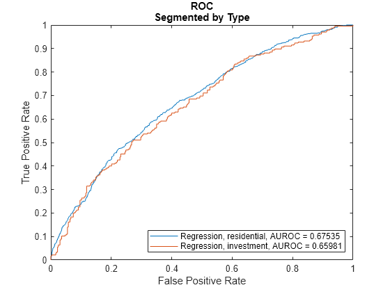

Figure contains an axes object. The axes object with title ROC Segmented by Type, xlabel False Positive Rate, ylabel True Positive Rate contains 2 objects of type line. These objects represent Regression, residential, AUROC = 0.67535, Regression, investment, AUROC = 0.65981.

Use the modelCalibration function to evaluate the model performance.

[calMeasure,calData] = modelCalibration(LGDmodel,weightedData);
disp(calMeasure)

                  RSquared     RMSE      Correlation    SampleMeanError
                  ________    _______    ___________    _______________

    Regression    0.067776    0.29877      0.26034          0.11801

disp(head(calData))

    Observed     Predicted_Regression    Residuals_Regression    Weights
    _________    ____________________    ____________________    _______

     0.032659           0.062216               -0.029557           0.1  
      0.43564          0.0023048                 0.43334           0.1  
    0.0064766         0.00079603               0.0056806           0.1  
     0.007947          0.0030436               0.0049035           0.1  
            0         0.00034465             -0.00034465           0.1  
      0.14572          0.0069889                 0.13873           0.1  
     0.025688          0.0074025                0.018285           0.1  
     0.063182            0.19431                -0.13113             1

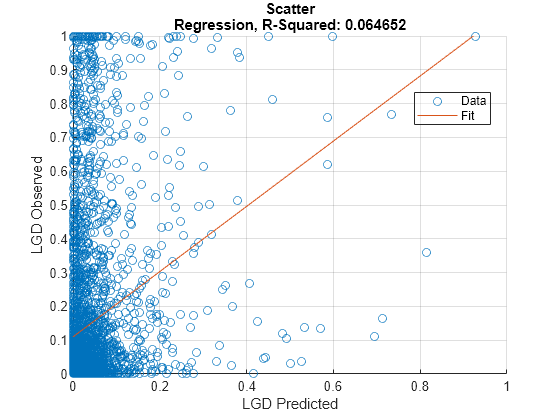
Use the modelCalibrationPlot function to visualize the observed LGD compared to the predicted LGD.

modelCalibrationPlot(LGDmodel,data)

Figure contains an axes object. The axes object with title Scatter Regression, R-Squared: 0.064652, xlabel LGD Predicted, ylabel LGD Observed contains 2 objects of type scatter, line. These objects represent Data, Fit.