Main Content

minjerkpolytraj

Generate minimum jerk trajectory through waypoints

Since R2021b

    Description

    [q,qd,qdd,qddd,pp,tPoints,tSamples] = minjerkpolytraj(waypoints,timePoints,numSamples) generates a minimum jerk polynomial trajectory that achieves a given set of input waypoints with their corresponding time points. The function returns positions, velocities, accelerations, and jerks at the given number of samples numSamples. The function also returns the piecewise polynomial pp form of the polynomial trajectory with respect to time, as well as the time points tPoints and the sample times tSamples.

    example

    [q,qd,qdd,qddd,pp,tPoints,tSamples] = minjerkpolytraj(___,Name=Value ) specifies options using one or more name-value pair arguments in addition to the input arguments from the previous syntax. For example, minjerkpolytraj(waypoints,timePoints,numSamples,VelocityBoundaryCondition=[1 0 -1 -1; 1 1 1 -1]) generates a two-dimensional minimum jerk trajectory and specifies the velocity boundary conditions in each dimension for each waypoint.

    [q,qd,qdd,qddd,pp,tPoints,tSamples] = minjerkpolytraj(___,TimeAllocation = true) optimizes a combination of jerk and total segment time cost. In this case, the function treats timePoints as an initial guess for the time of arrival at the waypoints.

    Examples

    collapse all

    Use the minjerkpolytraj function with a given set of 2-D xy waypoints. Time points for the waypoints are also given.

    wpts = [1 4 4 3 -2 0; 0 1 2 4 3 1];
    tpts = 0:5;

    Specify the number of samples in the output trajectory.

    numsamples = 100;

    Compute minimum jerk trajectories. The function outputs the trajectory positions (q), velocity (qd), acceleration (qdd), and jerks (qddd) at the given number of samples.

    [q,qd,qdd,qddd,pp,timepoints,tsamples] = minjerkpolytraj(wpts,tpts,numsamples);

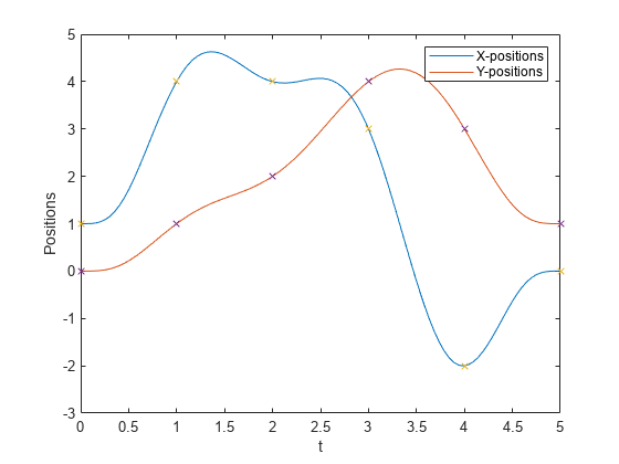
    Plot the trajectories for the x- and y-positions. Compare the trajectory with each waypoint.

    plot(tsamples,q)
    hold on
    plot(timepoints,wpts,'x')
    xlabel('t')
    ylabel('Positions')
    legend('X-positions','Y-positions')
    hold off

    Figure contains an axes object. The axes object with xlabel t, ylabel Positions contains 4 objects of type line. One or more of the lines displays its values using only markers These objects represent X-positions, Y-positions.

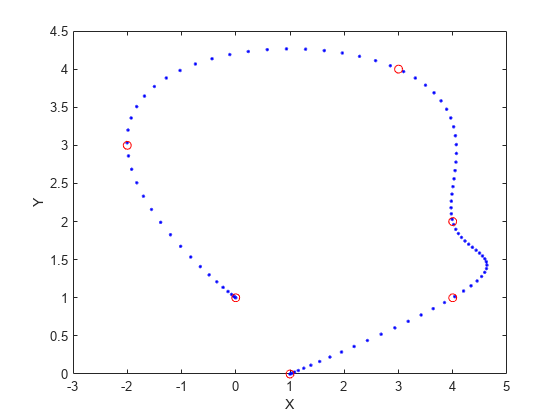
    You can also verify the actual positions in the 2-D plane. Plot the separate rows of the q vector and the waypoints as x- and y- positions.

    figure
    plot(q(1,:),q(2,:),'.b',wpts(1,:),wpts(2,:),'or')
    xlabel('X')
    ylabel('Y')

    Figure contains an axes object. The axes object with xlabel X, ylabel Y contains 2 objects of type line. One or more of the lines displays its values using only markers

    Input Arguments

    collapse all

    Waypoints for the trajectory, specified as an n-by-p matrix. n is the dimension of the trajectory, and p is the number of waypoints.

    Example: [2 5 8 4; 3 4 10 12]

    Data Types: single | double

    Time points for the waypoints of the trajectory, specified as a p-element row vector. p is the number of waypoints.

    Example: [1 2 3 5]

    Data Types: single | double

    Number of samples in the output trajectory, specified as a positive integer.

    Example: 50

    Data Types: single | double

    Name-Value Arguments

    Specify optional pairs of arguments as Name1=Value1,...,NameN=ValueN, where Name is the argument name and Value is the corresponding value. Name-value arguments must appear after other arguments, but the order of the pairs does not matter.

    Example: minjerkpolytraj(waypoints,timePoints,numSamples,VelocityBoundaryCondition=[1 0 -1 -1; 1 1 1 -1]) generates a two-dimensional minimum jerk trajectory and specifies the velocity boundary conditions in each dimension for each waypoint.

    Velocity boundary conditions for each waypoint, specified as an n-by-p matrix. Each row sets the velocity boundary for the corresponding dimension of the trajectory at each of p waypoints. By default, the function uses a value of 0 at the boundary waypoints and NaN at the intermediate waypoints.

    Example: VelocityBoundaryCondition=[1 0 -1 -1; 1 1 1 -1]

    Data Types: single | double

    Acceleration boundary conditions for each waypoint, specified as an n-by-p matrix. Each row sets the acceleration boundary for the corresponding dimension of the trajectory at each of p waypoints. By default, the function uses a value of 0 at the boundary waypoints and NaN at the intermediate waypoints.

    Example: AccelerationBoundaryCondition=[1 0 -1 -1; 1 1 1 -1]

    Data Types: single | double

    Jerk boundary conditions for each waypoint, specified as an n-by-p matrix. Each row sets the jerk boundary for the corresponding dimension of the trajectory at each of p waypoints. By default, the function uses a value of 0 at the boundary waypoints and NaN at the intermediate waypoints.

    Example: JerkBoundaryCondition=[1 0 -1 -1; 1 1 1 -1]

    Data Types: single | double

    Time allocation flag, specified as a logical 0 (false) or 1 (true). Enable this flag to optimize a combination of jerk and total segment time cost.

    Note

    If singularity occurs when the time allocation flag is enabled, reduce the MaxSegmentTime to MinSegmentTime ratio.

    Example: TimeAllocation=true

    Data Types: logical

    Weight for time allocation, specified as a positive scalar.

    Example: TimeWeight=120

    Data Types: single | double

    Minimum time segment length, specified as a positive scalar or (p1)-element row vector.

    Example: MinSegmentTime=0.2

    Data Types: single | double

    Maximum time segment length, specified as a positive scalar or (p1)-element row vector

    Example: MaxSegmentTime=10

    Data Types: single | double

    Output Arguments

    collapse all

    Positions of the trajectory at the given time samples in tSamples, returned as an n-by-m matrix. n is the dimension of the trajectory, and m is equal to numSamples.

    Velocities of the trajectory at the given time samples in tSamples, returned as an n-by-m matrix. n is the dimension of the trajectory, and m is equal to numSamples.

    Accelerations of the trajectory at the given time samples in tSamples, returned as an n-by-m matrix. n is the dimension of the trajectory, and m is equal to numSamples.

    Jerks of the trajectory at the given time samples in tSamples, returned as an n-by-m matrix. n is the dimension of the trajectory, and m is equal to numSamples.

    Piecewise-polynomial, returned as a structure that defines the polynomial for each section of the piecewise trajectory. You can build your own piecewise polynomials using mkpp, or evaluate the polynomial at specified times using ppval. The structure contains the fields:

    • form: 'pp'.

    • breaks: p-element vector of times when the piecewise trajectory changes forms. p is the number of waypoints.

    • coefs: n(p1)-by-order matrix for the coefficients for the polynomials. n(p1) is the dimension of the trajectory times the number of pieces. Each set of n rows defines the coefficients for the polynomial that described each variable trajectory.

    • pieces: p1. The number of breaks minus 1.

    • order: Degree of the polynomial + 1. The order of polynomial is 8.

    • dim: n. The dimension of the control point positions.

    Time points for the waypoints of the trajectory, returned as a p-element row vector. p is the number of waypoints.

    Time samples for the trajectory, returned as an m-element row vector. Each element of the output position q, velocity qd, acceleration qdd, and jerk qddd has been sampled at the corresponding time in this vector.

    References

    [1] Bry, Adam, Charles Richter, Abraham Bachrach, and Nicholas Roy. “Aggressive Flight of Fixed-Wing and Quadrotor Aircraft in Dense Indoor Environments.” The International Journal of Robotics Research, 34, no. 7 (June 2015): 969–1002.

    [2] Richter, Charles, Adam Bry, and Nicholas Roy. “Polynomial Trajectory Planning for Aggressive Quadrotor Flight in Dense Indoor Environments." Paper presented at the International Symposium of Robotics Research (ISRR 2013), 2013.

    Extended Capabilities

    C/C++ Code Generation
    Generate C and C++ code using MATLAB® Coder™.

    Version History

    Introduced in R2021b