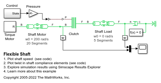
Flexible Shaft

Shaft with torsional and bending compliance

Libraries:
Simscape / Driveline / Couplings & Drives

Description

The Flexible Shaft block represents a driveline shaft with torsional and bending compliance. The shaft consists of a flexible material that twists in response to an applied torque and bends in response to static mass unbalance. The twisting action delays power transmission between the shaft ends, altering the dynamic response of the driveline system.

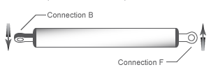
Illustration of a shaft with connection B at one end and connection F at the opposite end.

To represent a torsion-flexible shaft, the block uses a lumped mass method. This model divides the shaft into different elements that interconnect through parallel spring damper systems. The elements provide the shaft inertia while the spring damper systems provide the shaft compliance.

The block provides four parameterization methods that allow you to model compliance in either a homogeneous or an axially inhomogeneous shaft. An axially inhomogeneous shaft is one for which any of these attributes vary along the length of the shaft:

Torsional stiffness
Torsional inertia
Bending rigidity
Density
Shear modulus
Young's modulus
Outer diameter
Inner diameter

An additional parameter enables you to model the power losses in the bearings due to viscous friction at the shaft ends. For more information, see Torsion Model.

Note

The viscous friction at the shaft ends is different from the internal material damping, which corresponds to losses arising in the shaft material itself.

To represent the bending-flexible shaft, the block uses either a lumped mass method or an eigenmodes method. While the lumped mass method is simpler to configure, the eigenmodes method tends to simulate faster.

Tip

To prioritize simulation speed, first simulate using the lumped mass method, adjusting parameters as needed until the results match your mathematical models or experimental data. Next, simulate using the eigenmodes method. Again, adjust the parameters as needed until the results mathematical models or experimental data. For an example that uses both methods, see Shaft with Torsional and Transverse Flexibility.

For the lumped mass method, the number of bending shaft elements is the same as the number of torsion shaft elements. The model divides the shaft into a series of such elements. The elements provide the shaft inertia, while the stiffness matrices provide the shaft compliance. The eigenmodes method computes effective mass-spring-damper systems that represent the bending modes of the shaft. You can specify the number of modes to include and the precision of the mode shapes. Both the lumped mass and eigenmodes methods allow you to model:

Excitational static unbalances
Concentrically attached rigid masses
Up to four support locations along the shaft
Linear damping proportional to shaft inertia
Linear damping proportional to shaft stiffness

Note

The eigenmodes method assumes that the support damping is light compared to support stiffness.

Static unbalances, which excite bending, occur when the center of mass of the shaft or an attached rigid mass is not aligned with the shaft principal axis. You can vary the locations, magnitudes, and angle offsets of static unbalances on the shaft.

You can represent concentrically attached rigid masses as disks or idealized point masses. A concentric disk adds diametric and polar moments of inertia to the shaft and mass to the translation degree of freedom of the shaft nodes. The model assumes that the disk is thin, so the shaft can still bend on either side of the axial location with the disk. The polar moment of inertia couples the two planes of bending. A concentric point mass is an idealized version of a concentric disk. A concentric point mass adds mass to the translation degrees of freedom of the shaft nodes but does not have rotational moments of inertia. You can vary the locations and inertias of concentric disks or point masses that are attached to the shaft.

You can model the supports as ideal or by using stiffness and damping matrices. For each support, you can vary the:

Location — Any point along the shaft length.
Type — Ideal clamp, ideal pin, free, constant bearing stiffness and damping, or speed-dependent stiffness and damping.
Number — Two, three, or four.

For both bending methods, you can specify the shaft bending compliance by using either bending rigidity and linear mass density or Young’s modulus and shaft diameter.

You can parameterize the torsional model by using either stiffness k and inertia J or the dimensions and material properties of the shaft.

Torsion Model

For the torsion model, the Flexible Shaft block approximates the distributed, continuous properties of a shaft by using a lumped mass method. The model contains a finite number, N, of lumped inertia-damped spring elements in series, plus a final inertia. The result is a series of $N + 1$ inertias connected by N rotational springs and N rotational dampers.

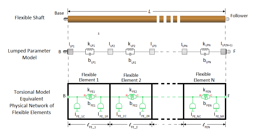
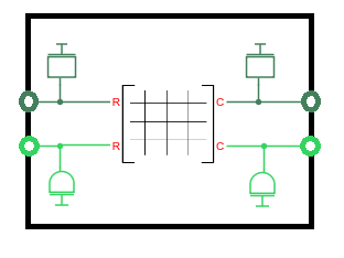
Diagram displaying how the flexible shaft breaks down into lumped parameters and further into torsional model equivalent systems of flexible elements.

The block treats the shaft as an equivalent physical network of N flexible elements. Each flexible element, FE_i, represents a short section of the driveshaft and contains:

One spring, k_{FE_i}, for torsional compliance. The network has a total of N springs.
One damper, b_{FE_i}, for material damping. The network has a total of N dampers.
Two inertias, I_{FE_iC} and I_{FE_iR}, for rotational resistance. The inertias of neighboring flexible elements are consolidated together so that the network has a total of $N + 1$ inertias.

For an axially homogeneous shaft, the flexible element lengths, compliance, damping, and distributed inertias in the physical network are equal, such that:

$l_{F E_1} = l_{F E_2} = \dots = l_{F E_N} = \frac{L}{N}$

$k_{F E_1} = k_{F E_2} = \dots = k_{F E_N} = k$

$b_{F E_1} = b_{F E_2} = \dots = b_{F E_N} = b$

$I_{F E_1C} = I_{F E_1R} = I_{F E_2C} = I_{F E_2R} = \dots = I_{F E_N C} = I_{F E_N R} = \frac{I}{2 N}$

For an axially inhomogeneous shaft, the amount of compliance, damping, and R-node and C-node inertia can differ for individual flexible elements in the physical network model.

Node Placement Algorithm

The balance between model fidelity and simulation speed depends on N, the number of flexible elements that the block uses to represent the shaft. For information on balancing simulation speed and model fidelity, see Improve Simulation Speed or Accuracy.

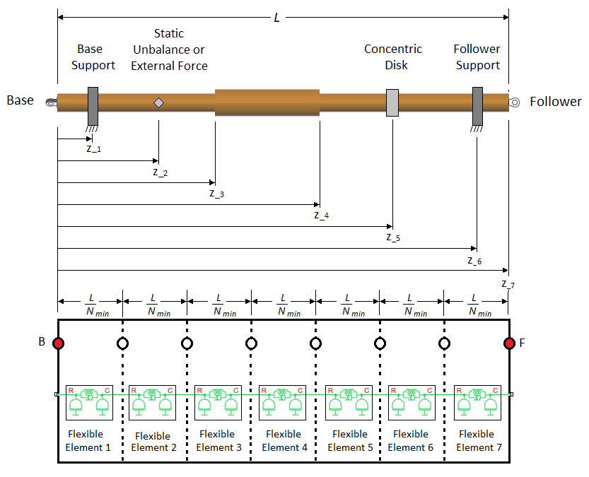
The block allows you to specify a minimum number of flexible elements, N_min, as the value for the Minimum number of flexible elements parameter. However, the number of flexible elements that the block actually uses depends on the complexity of the shaft that it is modeling. If the block requires more flexible elements than you specify to solve a model that contains axial inhomogeneity, intermediate supports, concentric disks or masses, static unbalances or external forces, then $N \geq N_{\min}$ .

For example, suppose that, for the complex shaft in the diagram, you specify axial locations for the supports, static unbalance or external force, larger diameter section, and concentric disk. You set the parameter for N_min to 7.

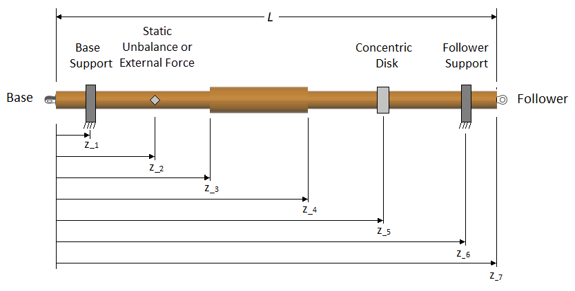
Illustration of a flexible shaft with the base, base support, static unbalance, concentric disc, follower support, and follower all labeled. The labels correspond to locations Z_1 through Z_7, respectively.

If model bending is on, the torsion model flexible element locations account for the locations of static unbalances or external forces and concentric rigid masses, so that the torsion flexible elements align with the bending flexible elements. During simulation, the torsion model is independent of any static unbalances, external forces, or concentric rigid masses.

The algorithm for the block determines the number of flexible elements and the length of the individual elements that are required to solve the simulation:

The block places one node at the base and follower ends of the shaft. These nodes are considered fixed in axial location because they represent physical entities along the shaft axis. In the diagram, fixed nodes are shown in red. The block evenly distributes the other five (N_min-2) internal nodes along the length of the shaft. It then places a flexible element between each consecutive pair of nodes.

For an end-supported, axially homogenous shaft, with no static unbalances, external forces, or attached concentric disks, depending on the other parameter options and values that you specify, the block might be able to solve the simulation using only N_min flexible elements of equivalent lengths:

$l = \frac{L}{N_{\min}}$
In most cases, however, the block can only solve the simulation if it adds more flexible elements.
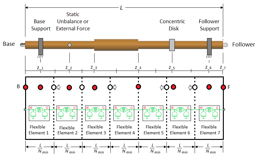
To add more flexible elements, the block places fixed internal nodes at these locations:
- Each shaft support location. The block allows you to specify the number and location of shaft supports. For the shaft in the diagram, there are supports at z₁ and z₆.
- Each static unbalance or external force. For the shaft in the diagram, there is a static unbalance at z₂.
- Each rigid mass. Rigid masses are concentrically attached disks or point masses. For the shaft in the diagram, there is a rigid mass, represented as a disk, at z₅.
- Each parameterization segment boundary. Parameterization boundaries are locations along an axially inhomogeneous shaft where two neighboring sections of the shaft vary in stiffness, inertia, or geometry. The block allows you to define the parameterization segment boundary locations. For the shaft in the diagram, there are segment boundaries at z₃ and z₄.
  
  Note that the block did not add a node at z₄ because a node was already added in the previous step of the algorithm. However, the node is now fixed because it represents a physical entity along the shaft length.
The block adjusts the nonfixed node locations between the fixed nodes so that they are evenly distributed.

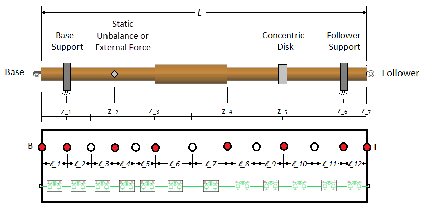
Finally, the block places flexible elements between each node. The length of each flexible element corresponds to the center-to-center distances between the neighboring nodes. The block distributes the inertia among the flexible elements based on the length of the individual element and the corresponding shaft geometry. Ultimately, this complex shaft is represented by 12 flexible elements, with $l_{1} = z_{1}$ , $l_{2} = l_{3} = \frac{(z_{2} - z_{1})}{2}$ , $l_{4} = l_{5} = \frac{(z_{3} - z_{2})}{2}$ , $l_{6} = l_{7} = \frac{(z_{4} - z_{3})}{2}$ , $l_{8} = l_{9} = \frac{(z_{5} - z_{4})}{2}$ , $l_{10} = l_{11} = \frac{(z_{6} - z_{5})}{2}$ , and $l_{12} = z_{7} - z_{6}$ .

If N_min is large enough to yield a number of unfixed nodes that is greater than the number of fixed nodes, the block distributes more than one unfixed node between each set of neighboring fixed nodes.

Dimensions and Material Properties

You can parameterize the torsion model by using either stiffness, k, and the polar moment of inertia, J, or the dimensions and material properties of the shaft.

The stiffness and inertia for each element are computed from the shaft dimensions and material properties as:

$J_{p} = \frac{π}{32} (D^{4} - d^{4})$

$m = \frac{π}{4} (D^{2} - d^{2}) ρ l$

$J = \frac{m}{8} (D^{2} + d^{2}) = ρ l \cdot J p$

$k = J p \cdot \frac{G}{l}$

where:

J_P is the polar moment of inertia of the shaft at the flexible element location.
D is the outer diameter of the shaft at the flexible element location.
d is the inner diameter of the shaft at the flexible element location. For a solid shaft, $d = 0$ . For an annular shaft, $d > 0$ .
$l$ is the flexible element length.
m is the mass of the shaft at the flexible element location.
J is the moment of inertia of the shaft at the flexible element location.
ρ is the density of the shaft material.
G is the shear modulus of elasticity of the shaft material.
k is the rotational stiffness of the flexible element.

Internal Material Damping

For either torsional parameterization, the internal material damping is defined by the damping ratio, c, for a single-flexible element model with the equivalent torsional stiffness and inertia. The damping coefficient is then $2 \frac{c k}{ω_{N}}$ , where the undamped natural frequency is $ω_{N} = \sqrt{\frac{2 k}{J}} .$ The damping torque applied across an individual flexible element of a lumped mass model is equivalent to the product of the damping coefficient and the relative rotational velocity of that flexible element.

Bending Models

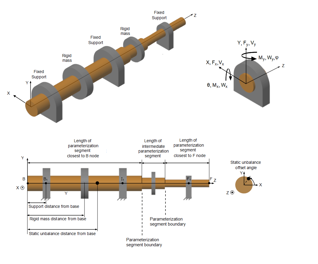
The Shaft Geometry, Support Loading, and Motion figure shows how to measure:

The static unbalance offset angle, which is the angle of a static unbalance about the shaft axis relative to the x axis
The distances of a support, a rigid mass, and a static unbalance, relative to the base end of the shaft, B
The parameterization of the segment lengths

In the figure, the shaft has three fixed supports:

B₁ — Base end support
I₁ — Intermediate support
F₁ — Follower end support

The shaft has translational velocity V, rotational velocity W, and exerts forces F, and moments M, on the supports. The curved arrows and sign conventions follow the right-hand rule. The signs of the physical signals that the block outputs correspond to the arrows that represent the forces, moments, and velocities of the shaft acting on the supports.

The vector signals are:

Force, $F r = [F_{x B 1}, F_{y B 1}, F_{x I 1}, F_{y I 1}, F_{x F 1}, F_{y F 1}]$
Moment, $M = [M_{x B 1}, M_{y B 1}, M_{x I 1}, M_{y I 1}, M_{x F 1}, M_{y F 1}]$
Translational velocity, $V = [V_{x B 1}, V_{y B 1}, V_{x I 1}, V_{y I 1}, V_{x F 1}, V_{y F 1}]$
Rotational velocity, $M = [M_{x B 1}, M_{y B 1}, M_{x I 1}, M_{y I 1}, M_{x F 1}, M_{y F 1}]$

If the shaft has two supports, each vector signal has a length of four. Force, for example, is then $F r = [F_{x B 1}, F_{y B 1}, F_{x F 1}, F_{y F 1}]$ .

If the shaft has four supports, each vector signal has a length of eight. Force, for example, is then $F r = [F_{x B 1}, F_{y B 1}, F_{x I 1}, F_{y I 1}, F_{x I 2}, F_{y I 2}, F_{x F 1}, F_{y F 1}]$ .

Shaft Geometry, Support Loading, and Motion

Diagram of shaft coordinates in a three-dimensional space.

Bending Model Lumped Mass Method

Like the torsion model, the lumped mass method for the bending model discretizes the distributed, continuous properties of the shaft into a finite number, N, of flexible elements. The N flexible elements correspond to $N + 1$ lumped inertias connected in series by damping and spring elements. However, for the bending model, each mass has four degrees of freedom: translation and rotation in both the x and y directions perpendicular to the shaft axis.

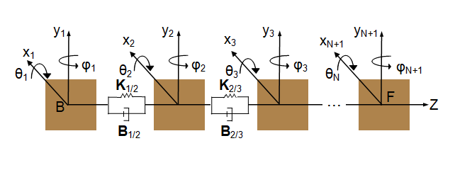
Bending model lumped mass discretization diagram.

The lumped mass equation of motion ^[1] is

$M \ddot{\vec{x}} + (B + G_{D i s k} Ω) \dot{\vec{x}} + (K + G_{D i s k} \dot{Ω}) \vec{x} = \vec{f} .$

where:

M is the $4 (N + 1) \times 4 (N + 1)$ matrix that represents the mass of the shaft.
B is the $4 (N + 1) \times 4 (N + 1)$ matrix for the internal damping and support damping.
G_Disk is the $4 (N + 1) \times 4 (N + 1)$ matrix that accounts for disk gyroscopics
Ω is the shaft torsional velocity during simulation.
K is the $4 (N + 1) \times 4 (N + 1)$ matrix for the spring stiffness.
$\vec{x}$ is the $4 (N + 1) \times 1$ vector that represents the degrees of freedom for all nodes.
$\vec{f}$ is the $4 (N + 1) \times 1$ vector that represents external forces due to the application of static mass unbalance.

The equation for the mass matrix [5] is

$M = M_{1 / 2} + M_{2 / 3} + \dots M_{i / i + 1} + \dots M_{N / N + 1} + \sum^{} M_{d i s k, i},$

where:

$M_{i / (i + 1)}$ is the mass matrix for an individual flexible element. For each flexible element, half of the mass and moment of inertia is transferred to the nodes at both ends of the flexible element. The $M_{i / (i + 1)}$ matrix has nonzero elements in the $(4 i - 3) : (4 i + 4)$ rows and the $(4 i - 3) : (4 i + 4)$ columns:

$M_{i / (i + 1)} = [\begin{matrix} 0 \\ ⋱ \\ \frac{1}{2} m & 0 & 0 & 0 & 0 & 0 & 0 & 0 \\ 0 & \frac{1}{2} m & 0 & 0 & 0 & 0 & 0 & 0 \\ 0 & 0 & I_{d} & 0 & 0 & 0 & 0 & 0 \\ 0 & 0 & 0 & I_{d} & 0 & 0 & 0 & 0 \\ 0 & 0 & 0 & 0 & \frac{1}{2} m & 0 & 0 & 0 \\ 0 & 0 & 0 & 0 & 0 & \frac{1}{2} m & 0 & 0 \\ 0 & 0 & 0 & 0 & 0 & 0 & I_{d} & 0 \\ 0 & 0 & 0 & 0 & 0 & 0 & 0 & I_{d} \\ ⋱ \\ 0 \end{matrix}],$
where:
- $l$ is the flexible element length along the shaft between internal nodes. To determine the length of each flexible element, the block uses the algorithm that is described in Node Placement Algorithm. Each flexible element contains two inertias. Each inertia has two translational degrees of freedom, two rotational degrees of freedom, and one stiffness matrix.
  Each flexible element in the equivalent physical model for bending in the XZ-plane (the beam translation in the X-direction and rotation about the Y-axis) and in the physical model for bending in the YZ-plane (the beam translation in the Y-direction and rotation about the X-axis) then contains two masses, two inertias, and a stiffness matrix.
  
  To determine the internal node locations, and therefore the number and lengths of the flexible elements, the block uses the same node-placement algorithm as it uses for the torsion model. For more information, see Node Placement Algorithm.
- m is the flexible element mass. m depends on the outer, D, and inner, d, diameters, the density, ρ, of the shaft and the length of the flexible element, such that $m = (\frac{π}{4}) (D^{2} - d^{2}) ρ l$ .
- I_d, the half-element mass moment of inertia about an axis perpendicular to the shaft axis, depends on the mass, m, length, $l$ , and torsion moment of inertia, J, of the flexible element, such that $I_{d} = \frac{J}{4} + \frac{m}{6} {(\frac{l}{2})}^{2}$ .
$\sum^{} M_{d i s k, i}$ is the summed mass matrices of the rigid masses concentrically attached to the shaft.
The mass properties of each rigid mass that is concentrically attached to the shaft are added to the closest node, $i$ , such that

$M_{d i s k, i} ([(4 i - 3) : 4 i], [(4 i - 3) : 4 i]) = [\begin{matrix} M_{d i s k, i} & 0 & 0 & 0 \\ 0 & M_{d i s k, i} & 0 & 0 \\ 0 & 0 & I_{D, d i s k, i} & 0 \\ 0 & 0 & 0 & I_{D, d i s k, i} \end{matrix}],$
where I_D,disk,i is the mass diametric moment of inertia about an axis perpendicular to the shaft for a rigid disk attached to the i^th node. The model assumes that the disk is thin, so the shaft can still bend on either side of the axial location with the disk. A concentric point mass has $I_{D, d i s k, i} = 0$ .

The equation for the damping matrix is

$B = α M + β K + B_{s u p p o r t},$

where:

α is the damping constant proportional to mass.
β is the damping constant proportional to stiffness.
B_support is the damping coefficient at each support. For a support at the i^th node, the damping matrix, in terms of global coordinates, is

$B_{s u p p o r t} ([(4 i - 3) : 4 i], [(4 i - 3) : 4 i]) = [\begin{matrix} b_{x x} & b_{x y} & 0 & 0 \\ b_{y x} & b_{y y} & 0 & 0 \\ 0 & 0 & b_{θ θ} & 0 \\ 0 & 0 & 0 & b_{φ φ} \end{matrix}],$
where:
- $[b_{x x} b_{x y} b_{y x} b_{y y}]$ is the support translational damping.
- $[b_{θ θ} b_{φ φ}]$ is the support rotational damping.
$G_{d i s k, i}$ accounts for the gyroscopic effects of any concentrically attached disks, and is defined as

$G_{d i s k, i} ([(4 i - 3) : 4 i], [(4 i - 3) : 4 i]) = [\begin{matrix} 0 & 0 & 0 & 0 \\ 0 & 0 & 0 & 0 \\ 0 & 0 & 0 & Ω I_{P, d i s k, i} \\ 0 & 0 & - Ω I_{P, d i s k, i} & 0 \end{matrix}],$
where I_P,disk,i is the mass polar moment of inertia about the shaft axis for the disk attached to the i^th node. The mass polar moment of inertia for a concentric point mass is $I_{P, d i s k, i} = 0$ .

The equation for the bearing stiffness matrix is

$K = K_{1 / 2} + K_{2 / 3} + ... + K_{N / N + 1} + \sum^{} K_{support},$

where:

$K_{i / i + 1}$ is the stiffness matrix for an individual shaft flexible element. The stiffness matrix for the $i^{t h}$ shaft flexible element, between the i^th and the ${(i + 1)}^{t h}$ nodes, has nonzero elements in the $(4 i - 3) : (4 i + 4)$ rows and the $(4 i - 3) : (4 i + 4)$ columns, such that

$K_{i / i + 1} = \frac{2 E I}{l^{3}} [\begin{matrix} 0 \\ ⋱ \\ 6 & 0 & 0 & 3 l & - 6 & 0 & 0 & 3 l \\ 0 & 6 & - 3 l & 0 & 0 & - 6 & - 3 l & 0 \\ 0 & - 3 l & 2 l^{2} & 0 & 0 & 3 l & l^{2} & 0 \\ 3 l & 0 & 0 & 2 l^{2} & - 3 l & 0 & 0 & l^{2} \\ - 6 & 0 & 0 & - 3 l & 6 & 0 & 0 & - 3 l \\ 0 & - 6 & 3 l & 0 & 0 & 6 & 3 l & 0 \\ 0 & - 3 l & l^{2} & 0 & 0 & 3 l & 2 l^{2} & 0 \\ 3 l & 0 & 0 & l^{2} & - 3 l & 0 & 0 & 2 l^{2} \\ ⋱ \\ 0 \end{matrix}],$

where:
- $l$ is the flexible element length.
- EI is the shaft rigidity.
K_support is the stiffness at each support. For a support at the i^th node, the stiffness matrix, in terms of global coordinates, is

$K_{s u p p o r t} ([(4 i - 3) : 4 i], [(4 i - 3) : 4 i]) = [\begin{matrix} k_{x x} & k_{x y} & 0 & 0 \\ k_{y x} & k_{y y} & 0 & 0 \\ 0 & 0 & k_{θ θ} & 0 \\ 0 & 0 & 0 & k_{φ φ} \end{matrix}],$
where:
- $[k_{x x} k_{x y} k_{y x} k_{y y}]$ is the support translational stiffness.
- $[k_{θ θ} k_{φ φ}]$ is the support rotational stiffness.

The support stiffness matrix, K_support, is nonzero only if you select Bearing matrix or Speed-dependent bearing matrix for the support. If you select the Clamped mounting type, the kinematic conditions of zero rotation and translation are applied to the degrees of freedom that correspond to the support node (B1, I1, I2, or F1). If you select the Pinned mounting type, the kinematic conditions of zero translation are applied to the translational degrees of freedom that correspond to the support node (B1, I1, I2, or F1).

The table includes the boundary conditions applied to the lumped mass nodes with supports.

Support Type	Boundary Condition for the Lumped Mass Equation
`Clamped`	$x_{i} = 0, y_{i} = 0, θ_{i} = 0, φ_{i} = 0$
`Pinned`	$x_{i} = 0, y_{i} = 0$
`Bearing Matrix`	K_support is nontrivial.
`Speed-dependent bearing matrix`	K_support is nontrivial and depends on shaft rotation speed. At each time step, K_Support is calculated as: $K_{S u p p o r t} (Ω) = l o o k u p (\| Ω_{R e f} \|, K_{S u p p o r t, R e f}, Ω, i n t e r p o l a t i o n = l i n e a r, e x t r a p o l a t i o n = n e a r e s t),$ where: Ω_Ref is the bearing speed, as specified, in the Supports settings, for the Bearing speed [s1,...,sS] parameter. For each support, K_Support,Ref is the bearing speed-dependent translational stiffness, which you specify in the Supports settings. The lookup table uses linear interpolation and nearest extrapolation for the shaft rotation speed.

The matrix that represents the degrees of freedom for all nodes, $\vec{x}$ , is calculated such that the degrees of freedom for the i^th and the ${(i + 1)}^{t h}$ nodes are

$\vec{x} = [\begin{matrix} \begin{matrix} \begin{matrix} \begin{matrix} ⋮ \\ \begin{matrix} x_{i} \\ y_{i} \\ θ_{i} \end{matrix} \\ φ_{i} \\ \begin{matrix} \begin{matrix} x_{i + 1} \\ y_{i + 1} \\ θ_{i + 1} \end{matrix} \\ φ_{i + 1} \\ ⋮ \end{matrix} \end{matrix} \end{matrix} \end{matrix} \end{matrix}] .$

External forces due to each static mass unbalance are applied to the closest node. The forcing at the $i^{t h}$ node is

${\vec{f}}_{4 (i - 1 : i - 2)} = [\begin{matrix} m ε_{j, o f f s e t} (Ω^{2}_{i} \cos (φ_{s h a f t, i} + φ_{o f f s e t, j}) + \frac{\partial Ω_{i}}{\partial t} \sin (φ_{s h a f t, i} + φ_{o f f s e t, j})) \\ m ε_{j, o f f s e t} (Ω^{2}_{i} \sin (φ_{s h a f t, i} + φ_{o f f s e t, j}) - \frac{\partial Ω_{i}}{\partial t} \cos (φ_{s h a f t, i} + φ_{o f f s e t, j})) \end{matrix}],$

where:

mε_j is the j^thstatic unbalance, located at the i^thnode.
Ω_i is the shaft rotational velocity during simulation for the i^th node.
φ_{shaft, i} is the torsion lumped mass rotation angle for the i^th node.

When the block models an external force that excites the shaft at a multiple or fraction of the rotation speed:

${\vec{f}}_{4 (i - 1 : i - 2)} = [\begin{matrix} F_{m a g, j} \cos (p ϕ_{s h a f t, j} + ϕ_{f_{o f f s e t}, j}) \\ F_{m a g, j} \cos (p ϕ_{s h a f t, j} + ϕ_{f_{o f f s e t}, j}) \end{matrix}],$

where:

F_mag,j is the j^th element of the External force magnitudes vector parameter.
p is the j^th element of the External force frequency harmonic of rotor speed vector parameter.
ϕ_{f_offset} is the j^th element of the External force offset angles vector parameter.
The node index i is the node at the z-axial position of the force.

Bending Model Eigenmodes Method

For the eigenmodes method, the block reduces the bending dynamics from the $4 (N + 1)$ degrees of freedom that the bending model lumped mass method provides, to M degrees of freedom, where M is the number of modes.

The block computes the bending mode properties of the shaft during model compilation, then solves the modal mass-spring-damper systems during model simulation.

Reducing the degrees of freedom in the model dynamics and separating the calculations into compile-time and run-time tasks improves simulation performance. The eigenmodes method assumes the mode shapes are unaffected by damping. Therefore, the method is best suited to models that include limited disk gyroscopic and support damping.

During compilation, the block computes the approximate damped eigenmodes using these steps:

The block computes the matrices using the same lumped mass equation of motion that it uses for the bending model lumped mass method:

$M \ddot{\vec{x}} + (B + G_{D i s k} Ω) \dot{\vec{x}} + (K + G_{D i s k} \dot{Ω}) \vec{x} = \vec{f} .$
For more information, see Bending Model Lumped Mass Method.
When determining the node axial locations for $\vec{x}$ , the block uses one of two variations of the Node Placement Algorithm that it uses for the torsion model and the bending model lumped mass method. The variation that the block uses depends on whether, in the Advanced Bending settings, the Bending mode determination parameter is set to Simscape determined or to User defined.
If the Bending mode determination parameter is set to Simscape determined, instead of using the Minimum number of flexible elements parameter for N_min, as the lumped mass methods do, the eigenmodes method calculates N_min as

$N_{M i n, E i g} = r o u n d (\frac{L}{d z}),$
where:
- L is the specified value of the Shaft length parameter.
- dz is the specified value of the Shaft length increments for mode shape computations parameter.
To compute the m undamped eigenmodes and eigenfrequencies, the block uses the eigs function. The equation takes the form :
```
[H_Right, λ] = eigs( sparse(K), sparse(M), mMax, 'smallestabs’ )
[H_Left, λ] = eigs( sparse(K), sparse(M), mMax, 'smallestabs’ )
```
where:
- H_Right is the $4 (N + 1) \times M$ right eigenvector matrix. Each column is a right eigenmode in the $\vec{x}$ coordinates.
- H_Left is the $4 (N + 1) \times M$ left eigenvector matrix. Each column is a left eigenmode in the $\vec{x}$ coordinates.
- λ represents the eigenvalues, which are the squares of the eigenfrequencies.
- m_Max is the Limit number of modes parameter.
The number of eigenmodes computed, m, is less than m_Max if:
- There are modes with eigenfrequencies that exceed the specified value for the Eigenfrequency upper limit parameter. The block discards these modes.
- The eigenvalues fail to converge. For more information, see eigs.
If you set Bending mode determination to User defined, the block computes the eigenvector matrix H for these parameters:
- X-direction mode shapes
- Y-direction mode shapes
- Shaft position
To determines the node axial locations for $\vec{x}$ , the block uses the elements specified for the Shaft position parameter as the primary nodes.
To compute the modal rotation, θ and φ, for each node, the block uses the gradient function. The equations take the form:
```
θ = -gradient(Y direction mode shapes)
φ = gradient(X direction mode shapes)
```
The block assembles the values from the X-direction mode shapes parameter, Y-direction mode shapes parameter, and modal rotations, θ and φ, into $\vec{x}$ coordinates for each column of H_Left and H_Right.
The block computes the modal matrices, M_Modal, K_Modal, B_Modal, G_Modal, and f_Modal, as:
$M_{M o d a l} = H_{L e f t}^{T} M H_{R i g h t}$
$K_{M o d a l} = H_{L e f t}^{T} K H_{R i g h t}$
$B_{M o d a l} = H_{L e f t}^{T} B H_{R i g h t}$
$G_{M o d a l} = H_{L e f t}^{T} G_{D i s k} H_{R i g h t}$
${\vec{f}}_{M o d a l} = H_{L e f t}^{T} \vec{f}$
Although the block computes undamped eigenmodes, H, in step 1, the modal damping matrix, B_Modal, and modal gyroscopics matrix, G_Modal, may model light damping. The block normalizes the matrices so that M_Modal is the identity matrix.

During simulation, the block simulates the eigenmode equation of motion:

$M_{M o d a l} \ddot{\vec{η}} + (B_{M o d a l} + G_{M o d a l} Ω) \dot{\vec{η}} + (K_{M o d a l} + G_{M o d a l} \dot{Ω}) \vec{η} = {\vec{f}}_{M o d a l},$

where the modal degrees of freedom, $\vec{η}$ , relate to the node degrees of freedom by:

$\vec{x} = H_{R i g h t} \vec{η}$

Speed-Dependent Eigenmodes Method

The support stiffness and support damping vary if, in the Supports settings, the mounting type parameter for any of the supports is set to Speed-dependent bearing matrix. The speed-dependent eigenmodes model accounts for these effects by varying the modal properties, H_Right and H_Left, B_Modal, G_Modal, K_Modal, and f_Modal as the shaft speed changes. M_Modal is normalized to the identity matrix for all shaft speeds, so it does not depend on shaft speed.

If the shaft has speed-dependent bearing supports, then the block repeats the bending mode eigenmodes method steps for each element in the shaft speed vector. The shaft vector elements are the specified values, in the Supports settings, for the Bearing speed [s1,...,sS] parameter. During simulation, the modal stiffness, damping, and forcing magnitude are adjusted based on lookup tables of the properties versus the shaft speed.

That is, the block simulates the eigenmode equation of motion as:

$M_{M o d a l} \ddot{\vec{η}} + (B_{M o d a l} (Ω) + G_{M o d a l} (Ω) Ω) \dot{\vec{η}} + (K_{M o d a l} (Ω) + G_{M o d a l} (Ω) \dot{Ω}) \vec{η} = {\vec{f}}_{M o d a l} (Ω),$

where K_Modal, B_Modal, and f_Modal have the form:

$K_{M o d a l} (Ω) = l o o k u p (| Ω_{R e f} |, K_{M o d a l, R e f}, Ω, i n t e r p o l a t i o n = l i n e a r, e x t r a p o l a t i o n = n e a r e s t),$

$B_{M o d a l} (Ω) = l o o k u p (| Ω_{R e f} |, B_{M o d a l, R e f}, Ω, i n t e r p o l a t i o n = l i n e a r, e x t r a p o l a t i o n = n e a r e s t),$

$G_{M o d a l} (Ω) = l o o k u p (| Ω_{R e f} |, G_{M o d a l, R e f}, Ω, i n t e r p o l a t i o n = l i n e a r, e x t r a p o l a t i o n = n e a r e s t),$

${\vec{f}}_{M o d a l} (Ω) = l o o k u p (| Ω_{R e f} |, {\vec{f}}_{M o d a l, R e f}, Ω, i n t e r p o l a t i o n = l i n e a r, e x t r a p o l a t i o n = n e a r e s t),$

where:

Ω_Ref is the specified value, in the Supports settings, for the Bearing speed [s1,...,sS] parameter.
K_Modal,Ref is the table of modal stiffnesses at each Ω_Ref.
B_Modal,Ref is the table of support damping at each Ω_Ref.
G_Modal,Ref is the table of disk gyroscopic damping at each Ω_Ref.
f_Modal,Ref is the table of modal forcing at each Ω_Ref.

The block correlates the mode shape similarity at different values of Ω_Ref and reorders modes, if necessary, so that each modal degree of freedom, $\vec{η}$ , has properties that gradually change with the shaft speed.

Improve Simulation Speed or Accuracy

The balance between simulation accuracy and performance depends on N, the number of flexible elements that the block uses to represent the shaft. Simulation accuracy is a measure of how much the simulation results agree with mathematical and empirical models. Generally, as N increases, so does model fidelity and simulation accuracy. However, the computational cost of the simulation is also correlated to N, and as computational cost increases, performance decreases. Conversely, as N decreases, simulation speed increases but simulation accuracy decreases.

To increase simulation accuracy for the lumped mass method for either a torsion or bending model, increase the minimum number of flexible elements, N_min. The single-flexible-element torsion model exhibits a torsional eigenfrequency that is close to the first eigenfrequency of the continuous, distributed parameter model. For greater accuracy you can select 2, 4, 8, or more flexible elements. For example, the four lowest torsional eigenfrequencies are represented with an accuracy of 0.1, 1.9, 1.6, and 5.3 percent, respectively, by a 16-flexible-element model.

To increase simulation accuracy for the eigenmodes method to a bending model:

If simulating with static eigenmode dependency on rotation speed, verify that the Nominal shaft speed for bending modes parameter is close to the simulation shaft speed. This parameter may affect model results if you parameterize a rigid disk attached to the shaft with a large mass moment of inertia about the shaft axis or specify any speed-dependent bearing matrix supports.
If simulating with dynamic eigenmode dependency on rotation speed, verify that, in the Supports settings, the specified values for the Bearing speed [s1,...,sS] span the shaft speed range of the simulation or that saturation of the support stiffness and damping at shaft speeds outside the range is an acceptable approximation.
In the Advanced Bending settings, decrease the value of the Shaft length increments for mode shape computations parameter. Reducing the value can increase the accuracy of modal frequencies and shapes.
Decrease the support damping and disk polar moment of inertia about the shaft axis. Simscape™ computations of the mode shapes and frequencies before simulation do not account for this damping.
Check the sensitivity to the Advanced Bending settings by using your parameters in the flexible shaft model in the Shaft with Torsional and Transverse Flexibility example. Adjust the parameters and use the links provided in the example to examine how the values affect the eigenmode frequencies and shapes. Adjust the parameter values in your model accordingly.
Increase the values of the Eigenfrequency upper limit and Limit number of modes parameters. The highest modal frequency in the simulation must be significantly larger than the shaft rotation frequency.

Assumptions and Limitations

The distributed parameter model of a continuous torsional shaft is approximated by a finite number, N, of lumped masses.
Shaft rotation and torsion flexibility excite shaft bending, but bending does not affect shaft rotation and torsion flexibility.
Rigid point masses or disks attached to the shaft have thin lengths parallel to the shaft axis.
For the eigenmodes bending model, damping does not affect the eigenfrequencies.
Shaft bending is not transmitted between Flexible Shaft blocks.
Relative to the shaft length, the shaft outer diameter is small.
Relative to the shaft length, the bending deflection is small.
Static mass unbalances are the only shaft-bending external exciting loads.
Shaft supports are stationary.
Gyroscopic effects of the rigid disks are considered; gyroscopic effects of the shaft itself are neglected.
Static mass unbalance forcing in the eigenmodes method uses the rotation speed at the shaft midpoint.
If the shaft models torsion only and uses the parameterization options By stiffness and inertia or By segment stiffness and inertia, the block uses only two supports, one each at the B and F ends.

Examples

Flexible Shaft

Two flexible aluminum shafts modeled using a lumped parameter approach. Both shafts consist of 20 segments containing inertias, damping, and stiff torsional springs. At the start of the simulation, the clutch is unlocked and the driven shaft is free. Note that the initial velocity of the motor shaft is set to 200 rad/s and that the system starts at steady state. The clutch engages and disengages during the test, and during each event the effect of the shaft flexibility can be seen in the simulation results.

Open Model

Wind Turbine Driveline with Vibrations

A wind turbine rotor, controller, and flexible drive shaft with transverse vibrations. Click the button below to open the model.

Open Live Script

Ports

Output

expand all

Fr — Force on bearing supports
physical signal

Physical signal outport associated with the force that the shaft exerts on the bearing supports.

Dependencies

To enable this port, set Model bending to On.

M — Moment on bearing supports
physical signal

Physical signal outport associated with the moment that the shaft exerts on the bearing supports.

Dependencies

To enable this port, set Model bending to On.

V — Shaft translational velocity
physical signal

Physical signal outport associated with the translational velocity of the shaft at the bearing supports.

Dependencies

To enable this port, set Model bending to On.

W — Shaft angular velocity
physical signal

Physical signal outport associated with the angular velocity of the shaft at the bearing supports.

Dependencies

To enable this port, set Model bending to On.

Conserving

expand all

B — Base
rotational mechanical

Rotational conserving port associated with the shaft base.

F — Follower
rotational mechanical

Rotational conserving port associated with the shaft follower.

Parameters

expand all

Shaft

Model torsional flexibility — Torsional flexibility option
`on` (default) | `off`

Whether to model torsional flexibility.

Model bending flexibility — Bending flexibility option
`off` (default) | `on`

Whether to model bending flexibility.

Minimum number of flexible elements — Minimum number of flexible elements
`1` (default) | positive integer

Minimum number of flexible elements, N_min, for the approximation.

It is possible that the flexible elements have different lengths or that the simulated number of flexible elements, N, is larger than N_min. For more information, see Node Placement Algorithm.

A larger number of flexible elements, N, increases the fidelity of the model, but reduces simulation performance. The single flexible element model (N=1) exhibits a torsion eigenfrequency that is close to the first eigenfrequency of the continuous, distributed parameter model.

If model fidelity is more important than performance, select 2, 4, 8, or more flexible elements. For example, the four lowest torsion eigenfrequencies are represented with an accuracy of 0.1, 1.9, 1.6, and 5.3 percent, respectively, by a model with 16 flexible elements. Generally, more flexible elements are required for accurately modeling bending dynamics than are required for accurately modeling torsion dynamics.

For more information, see Improve Simulation Speed or Accuracy.

Dependencies

To enable this parameter, select either Model torsional flexibility or Model bending flexibility.

Parameterization — Parameterization method
`By stiffness and inertia` (default) | `By material and geometry` | `By segment stiffness and inertia` | `By material and segment geometry`

Parameterization method. You can model a homogeneous shaft or one that is axially inhomogeneous for any of these attributes:

Torsional stiffness
Torsional inertia
Bending rigidity
Density
Shear modulus
Young's modulus
Outer diameter
Inner diameter

Select from these homogeneous shaft parameterizations:

By stiffness and inertia — Specify the torsional stiffness and inertia, and the density per unit length of the shaft. For the bending model, also specify the bending rigidity and length of the shaft.
By material and geometry — Specify the length and axial cross-sectional geometry, in terms of inner and outer diameters, of the shaft. For the shaft material, specify the density and shear modulus. For the bending model, also specify Young's modulus for the material of the shaft.

The parameterization options for an axially inhomogeneous shaft model are:

By segment stiffness and inertia — For each segment of the shaft, specify the torsional stiffness, torsional inertia, and density per unit length. For the bending model, also specify the bending rigidity and length for each segment.
By material and segment geometry — For each segment of the shaft, specify the length and axial cross-sectional geometry, in terms of inner and outer diameters. For the material of the shaft, specify the density and shear modulus. For the bending model, also specify Young's modulus for the material of the shaft.

Shaft length — Shaft length
`1` `m` (default) | positive scalar

Length of the shaft.

Dependencies

To enable this parameter, choose one of these options:

Set Parameterization to By material and geometry .
Select Model bending flexibility, and set Parameterization to By stiffness and inertia or By material and geometry.

Segment lengths [B,...,F] — Length of each shaft segment
`[1, .5, .25]` (default) | vector

Length of each shaft segment that the shaft is divided into lengthwise for modeling an axially inhomogeneous shaft. The number of elements in the vector is equal to the number of segments that you use to model the inhomogeneous shaft. The order of the elements in the vector corresponds to the segment order relative to B, the base end of the shaft.

Dependencies

To enable this parameter, choose one of these options:

Set Parameterization to By material and segment geometry.
Select Model bending flexibility, and set Parameterization to By segment stiffness and inertia.

Torsional stiffness — Material stiffness
`2e5` `N*m/rad` (default) | positive scalar

Torque per radian twist of the shaft.

Dependencies

To enable this parameter, select Model torsional flexibility and set Parameterization to By stiffness and inertia.

Torsional Inertia — Polar moment of inertia
`0.02` `kg*m^2` (default) | positive scalar

Ability of the shaft to resist torsional acceleration.

Dependencies

To enable this parameter, set Parameterization to By stiffness and inertia.

Segment torsional stiffness [B,...,F] — Material stiffness for each shaft segment
`[400000, 200000, 100000]` `N*m/rad` (default) | positive vector

Torque per radian twist for each segment of the shaft. The number of elements in the vector must be the same as the number of elements specified for the Segment lengths [B,...,F] parameter. The order of the elements in the vector corresponds to the segment order relative to B, the base end of the shaft.

Dependencies

To enable this parameter, set Parameterization to By segment stiffness and inertia.

Segment torsional inertia [B,...,F] — Polar moment of inertia for each shaft segment
`[.025, .02, .015]` `kg*m^2` (default) | positive vector

Ability of the each shaft segment to resist torsional acceleration. The number of elements in the vector must be the same as the number of elements specified for the Segment lengths [B,...,F] parameter. The order of the elements in the vector corresponds to the segment order relative to, B, the base end of the shaft.

Dependencies

To enable this parameter, set Parameterization to By segment stiffness and inertia.

Bending rigidity — Bending rigidity
`5e5` `m^4*Pa` (default) | positive scalar

Bending rigidity for the shaft material.

Dependencies

To enable this parameter, select Model bending flexibility, and set Parameterization to By stiffness and inertia.

Linear density — Density per unit length
`19` `kg/m` (default) | positive scalar

Density of the shaft material per unit length of the shaft.

Dependencies

To enable this parameter, select Model bending flexibility, and set Parameterization to By stiffness and inertia.

Segment bending rigidity [B,...,F] — Bending rigidity of each segment
`[600000, 500000, 400000]` `m^4*Pa` (default) | vector of positive elements

Bending rigidity for the material of each sequential segment of the shaft. The number of elements in the vector must be the same as the number of elements specified for the Segment lengths [B,...,F] parameter. The order of the elements in the vector corresponds to the segment order relative to B, the base end of the shaft.

Dependencies

To enable this parameter, select Model bending flexibility, and set Parameterization to By stiffness and inertia.

Segment linear density [B,...,F] — Density per unit length for each segment
`[20, 19, 18]` `kg/m` (default) | positive vector

Density of the shaft material per unit length of each segment of the shaft. The number of elements in the vector must be the same as the number of elements specified for the Segment lengths [B,...,F] parameter. The order of the elements in the vector corresponds to the segment order relative to B, the base end of the shaft.

Dependencies

To enable this parameter, set Parameterization to By segment stiffness and inertia.

Material density — Material density
`7.8e3` `kg/m^3` (default) | positive scalar

Density of the shaft material.

Dependencies

To enable this parameter, set Parameterization to By material and geometry or By material and segment geometry.

Shear modulus — Shear modulus
`7.93e9` `Pa` (default) | positive scalar

Shear modulus for the shaft material.

Dependencies

To enable this parameter, set Parameterization to By material and geometry or By material and segment geometry.

Shaft geometry — Cross-sectional geometry
`Solid` (default) | `Annular`

Cross-sectional geometry along the length of the shaft. If the shaft or segments of the shaft are hollow, select Annular. Otherwise, select Solid.

Dependencies

To enable this parameter, set Parameterization to By material and geometry or By material and segment geometry.

Young's modulus — Young's modulus
`200e9` `Pa` (default) | positive scalar

Young's modulus for the material.

Dependencies

To enable this parameter, select Model bending flexibility and set Parameterization to By material and geometry or By material and segment geometry.

Shaft outer diameter — Outer diameter of the shaft
`0.075` `m` (default) | positive scalar

Outer diameter of the shaft.

Dependencies

To enable this parameter, set Parameterization to By material and geometry.

Shaft inner diameter — Inner diameter of the shaft
`0.05` `m` (default) | positive scalar

Inner diameter of the annular shaft. The value must be smaller than the value specified for the Shaft outer diameter parameter.

Dependencies

To enable this parameter, set Parameterization to By material and geometry and set Shaft geometry to Annular.

Segment outer diameters [B,...,F] — Outer diameter for each shaft segment
`[.085, .075, .065]` `m` (default) | positive vector

Outer diameter of each shaft segment. The number of elements in the vector must be the same as the number of elements specified for the Segment lengths [B,...,F] parameter. The order of the elements in the vector corresponds to the segment order relative to B, the base end of the shaft.

Dependencies

To enable this parameter, set Parameterization to By material and segment geometry.

Segment inner diameters [B,...,F] — Inner diameter for each shaft segment
`[.055, .05, .045]` `m` (default) | vector

Inner diameters of the shaft segments. The number of elements in the vector must be the same as the number of elements specified for the Segment lengths [B,...,F] parameter. The order of the elements in the vector corresponds to the segment order relative to B, the base end of the shaft. Each value must be smaller than the corresponding value specified for the Segment outer diameter [B,...,F] parameter. If a shaft segment is solid, specify 0 for the corresponding vector element. At least one element in the vector must be positive.

Dependencies

To enable this parameter, set Parameterization to By material and segment geometry, and set Shaft geometry to Annular.

Torsion

Damping ratio from internal losses — Material damping ratio
`0.01` (default) | positive scalar

Material damping ratio.

Dependencies

To enable this parameter, select Model torsional flexibility.

Viscous friction coefficients at base (B) and follower (F) — Viscous friction coefficients
`[0, 0]` `N*m/(rad/s)` (default) | nonnegative vector

Viscous friction coefficients at the base, B, and follower, F, ends of the shaft. The vector must contain two elements.

Dependencies

To enable this parameter, deselect Model bending flexibility and set Parameterization to By stiffness and inertia or By segment stiffness and inertia.

Viscous friction coefficients at each support [B1,...,F1] — Viscous friction coefficients
`[0, 0]` `N*m/(rad/s)` (default) | nonnegative vector

Viscous friction coefficients at each support. The number of elements in the vector must be the same as the number specified in the Number of supports parameter. The order of the elements must correspond to the sequential position of each support B, the base end of the shaft.

Dependencies

To enable this parameter, choose one of these options:

Select Model bending flexibility.
Deselect Model bending flexibility and set Parameterization to By material and geometry or By material and segment geometry.

Initial shaft torsional deflection — Initial shaft torsional deflection
`0` `rad` (default) | nonnegative scalar

Angular deflection of the shaft at the start of simulation.

A positive initial deflection results in a positive rotation of B, the base end of the shaft, relative to F, the follower end of the shaft.

Dependencies

To enable this parameter, select Model torsional flexibility.

Initial shaft rotational velocity — Initial angular velocity
`0` `rpm` (default) | nonnegative scalar

Angular velocity of the shaft at the start of simulation.

Dependencies

To enable this parameter, select Model torsional flexibility.

Supports

To enable these parameters, choose one of these options:

Deselect Model bending flexibility, and set Parameterization to By material and geometry or By material and segment geometry.
Select Model bending flexibility.

Number of supports — Number of supports
`2` (default) | `3` | `4`

Number of shaft supports.

Dependencies

To enable these parameters, choose one of these options:

Deselect Model bending flexibility, and set Parameterization to By material and geometry or By material and segment geometry
Select Model bending flexibility.

Support locations relative to base (B) — Support locations
`[0, 1]` `m` (default) | nonnegative increasing vector

Support locations relative to B, the base end of the shaft. The number of elements must be the same as the number specified for the Number of supports parameter. The order of the elements corresponds to the sequential position of each support relative to the base end of the shaft. The largest value must be no larger than the length of the shaft. For a segmented shaft model, the shaft length is equal to the sum of the individual segment lengths.

Dependencies

Deselect Model bending flexibility, and set Parameterization to By material and geometry or By material and segment geometry
Select Model bending flexibility.

Base (B1) mounting type — Support B1 mounting type
`Clamped` (default) | `Pinned` | `Free` | `Bearing matrix` | `Speed-dependent bearing matrix`

Type of mounting at the base end of the shaft.

Dependencies

To enable this parameter, select Model bending flexibility.

Base (B1) rotational damping [xx,yy] — Support B1 rotational damping
`[1e3, 1e3]` `N*m/(rad/s)` (default) | vector

Rotational damping for the B1 support. B1 is the support that is closest to B, the base end of the shaft. The elements of the two-element vector are:

xx — Damping about the x-axis
yy — Damping about the y-axis

Dependencies

To enable this parameter, select Model bending flexibility, and set Base (B1) mounting type to Pinned, Free, Bearing matrix, or Speed-dependent bearing matrix.

Base (B1) translational damping [xx,xy,yx,yy] — Support B1 translational damping
`[2e4, -4.4e4, -4.4e4, 3.5e5]` `N/(m/s)` (default) | vector

Translational damping for the B1 support. The elements of the four-element vector are:

xx — Damping in the x-axis direction
xy — Damping in the x-axis direction coupled with motion in the y-axis direction
yx — Damping in the y-axis direction coupled with motion in the x-axis direction
yy — Damping in the y-axis direction

Dependencies

To enable this parameter, select Model bending flexibility, and set Base (B1) mounting type to Bearing matrix.

Base (B1) speed-dependent translational damping [xx1,xy1,yx1,yy1;...xxS,xyS,yxS,yyS] — Support B1 speed-dependent translational damping
`[2e4, -4.4e4, -4.4e4, 3.5e5; 1e4, -2.5e4, -2.5e4, 1.4e5; 5e3, -1.0e4, -1.0e4, 2.0e4]` `N/(m/s)` (default) | matrix

Speed-dependent translational damping for the B1 support. The number of rows in the matrix must equal the number of elements in the vector specified for the Bearing speed [s1, … sS] parameter. Each row contains four elements:

xx_s — Damping in the x-axis direction at the s^th speed
xy_s — Damping in the x-axis direction coupled with motion in the y-axis direction at the s^th speed
yx_s — Damping in the y-axis direction coupled with motion in the x-axis direction at the s^th speed
yy_s — Damping in the y-axis direction at the s^th speed

Dependencies

To enable this parameter, select Model bending flexibility, and set Base (B1) mounting type to Bearing matrix.

Base (B1) rotational stiffness [xx,yy] — Support B1 rotational stiffness
`[1e4, 1e4]` `N*m/rad` (default) | nonnegative vector

Rotational stiffness for the B1 support. The elements of the two-element vector are:

xx — Stiffness about the x-axis
yy — Stiffness about the y-axis

Dependencies

To enable this parameter, select Model bending flexibility, and set Base (B1) mounting type to Bearing matrix or Speed-dependent bearing matrix.

Base (B1) translational stiffness [xx,xy,yx,yy] — Support B1 translational stiffness
`[1e6, -2e5, -3e5, 5e]` `N/m` (default) | vector

Translational stiffness for the B1 support. The elements of the four-element vector are:

xx — Stiffness in the x-axis direction
xy — Stiffness in the x-axis direction coupled with motion in the y-axis direction
yx — Stiffness in the y-axis direction coupled with motion in the x-axis direction
yy — Stiffness in the y-axis direction

Dependencies

To enable this parameter, select Model bending flexibility, and set Base (B1) mounting type to Bearing matrix.

Base (B1) speed-dependent translational stiffness [xx1,xy1,yx1,yy1;...xxS,xyS,yxS,yyS] — Support B1 speed-dependent translational stiffness
`[1e6, -6e5, -3.5e6, 8e6; 1e6, -2e5, -3.0e6, 5e6; 1e6, -5e4, -2.5e6, 3e6]` `N/m` (default) | matrix

Speed-dependent translational stiffness for the B1 support. The number of rows in the matrix must equal the number of elements in the vector specified for the Bearing speed [s1, … sS] parameter. Each row contains four elements:

xx_s — Stiffness in the x-axis direction at the s^th speed
xy_s — Stiffness in the x-axis direction coupled with motion in the y-axis direction at the s^th speed
yx_s — Stiffness in the y-axis direction coupled with motion in the x-axis direction at the s^th speed
yy_s — Stiffness in the y-axis direction at the s^th speed

All xx and yy stiffness values must be positive. All xy and yx values must be zero or nonzero at all speeds.

Dependencies

To enable this parameter, select Model bending flexibility, and set Base (B1) mounting type to Speed-dependent bearing matrix.

Intermediate (I1) mounting type — Support I1 mounting type
`Clamped` (default) | `Pinned` | `Free` | `Bearing matrix` | `Speed-dependent bearing matrix`

Type of mounting at the I1 support. The I1 support is the closest intermediate support to the B1 support.

Dependencies

To enable this parameter, select Model bending flexibility, and set Number of supports to 3 or 4.

Intermediate (I1) rotational damping [xx,yy] — Support I1 rotational damping
`[1e3, 1e3]` `N*m/(rad/s)` (default) | vector

Rotational damping for the I1 support. The elements of the two-element vector are:

xx — Damping about the x-axis
yy — Damping about the y-axis

Dependencies

To enable this parameter:

Select Model bending flexibility.
Set Number of supports to 3 or 4.
Set Intermediate (I1) mounting type to Pinned, Free, Bearing matrix, or Speed-dependent bearing matrix.

Intermediate (I1) translational damping [xx,xy,yx,yy] — Support I1 translational damping
`[2e4, -4.4e4, -4.4e4, 3.5e5]` `N/(m/s)` (default) | vector

Translational damping for the I1 support. The elements of the four-element vector are:

xx — Damping in the x-axis direction
xy — Damping in the x-axis direction coupled with motion in the y-axis direction
yx — Damping in the y-axis direction coupled with motion in the x-axis direction
yy — Damping in the y-axis direction

Dependencies

To enable this parameter:

Select Model bending flexibility.
Set Number of supports to 3 or 4.
Set Intermediate (I1) mounting type to Bearing matrix.

Intermediate (I1) speed-dependent translational damping [xx1,xy1,yx1,yy1;...xxsS,xyS,yxS,yyS] — Support I1 speed-dependent translational damping
`[2e4, -4.4e4, -4.4e4, 3.5e5; 1e4, -2.5e4, -2.5e4, 1.4e5; 5e3, -1.0e4, -1.0e4, 2.0e4]` `N/(m/s)` (default) | matrix

Speed-dependent translational damping for the I1 support. The number of rows in the matrix must equal the number of elements in the vector specified for the Bearing speed [s1, … sS] parameter. Each row contains four elements:

xx_s — Damping in the x-axis direction at the s^th speed
xy_s — Damping in the x-axis direction coupled with motion in the y-axis direction at the s^th speed
yx_s — Damping in the y-axis direction coupled with motion in the x-axis direction at the s^th speed
yy_s — Damping in the y-axis direction at the s^th speed

Dependencies

To enable this parameter:

Select Model bending flexibility.
Set Number of supports to 3 or 4.
Set Intermediate (I1) mounting type to Bearing matrix.

Intermediate (I1) rotational stiffness [xx,yy] — Support I1 rotational stiffness
`[1e4, 1e4]` `N*m/rad` (default) | nonnegative vector

Rotational stiffness for the I1 support. The elements of the two-element vector are:

xx — Stiffness about the x-axis
yy — Stiffness about the y-axis

Dependencies

To enable this parameter:

Select Model bending flexibility.
Set Number of supports to 3 or 4.
Set Intermediate (I1) mounting type to Bearing matrix or Speed-dependent bearing matrix.

Intermediate (I1) translational stiffness [xx,xy,yx,yy] — Support I1 translational stiffness
`[1e6, -2e5, -3e5, 5e]` `N/m` (default) | vector

Translational stiffness for the I1 support. The elements of the four-element vector are:

xx — Stiffness in the x-axis direction
xy — Stiffness in the x-axis direction coupled with motion in the y-axis direction
yx — Stiffness in the y-axis direction coupled with motion in the x-axis direction
yy — Stiffness in the y-axis direction

Dependencies

To enable this parameter:

Select Model bending flexibility.
Set Number of supports to 3 or 4.
Set Intermediate (I1) mounting type to Bearing matrix.

Intermediate (I1) speed-dependent translational stiffness [xx1,xy1,yx1,yy1;...xxS,xyS,yxS,yyS] — Support I1 speed-dependent translational stiffness
`[1e6, -6e5, -3.5e6, 8e6; 1e6, -2e5, -3.0e6, 5e6; 1e6, -5e4, -2.5e6, 3e6]` `N/m` (default) | matrix

Speed-dependent translational stiffness for the I1 support. The number of rows in the matrix must equal the number of elements in the vector specified for the Bearing speed [s1, … sS] parameter. Each row contains four elements:

xx_s — Stiffness in the x-axis direction at the s^th speed
xy_s — Stiffness in the x-axis direction coupled with motion in the y-axis direction at the s^th speed
yx_s — Stiffness in the y-axis direction coupled with motion in the x-axis direction at the s^th speed
yy_s — Stiffness in the y-axis direction at the s^th speed

All xx and yy stiffness values must be positive. All xy and yx values must be zero or nonzero at all speeds.

Dependencies

To enable this parameter:

Select Model bending flexibility.
Set Number of supports to 3 or 4.
Set Intermediate (I1) mounting type to Speed-dependent bearing matrix.

Intermediate (I2) mounting type — Support I2 mounting type
`Clamped` (default) | `Pinned` | `Free` | `Bearing matrix` | `Speed-dependent bearing matrix`

Type of mounting at the I2 support. The I2 support is located between the I1 and F1 supports.

Dependencies

To enable this parameter, select Model bending flexibility, and set Number of supports to 4.

Intermediate (I2) rotational damping [xx,yy] — Support I2 rotational damping
`[1e3, 1e3]` `N*m/(rad/s)` (default) | vector

Rotational damping for the I2 support. The elements of the two-element vector are:

xx — Damping about the x-axis
yy — Damping about the y-axis

Dependencies

To enable this parameter:

Select Model bending flexibility.
Set Number of supports to 4.
Set Intermediate (I2) mounting type to Pinned, Free, Bearing matrix, or Speed-dependent bearing matrix.

Intermediate (I2) translational damping [xx,xy,yx,yy] — Support I2 translational damping
`[2e4, -4.4e4, -4.4e4, 3.5e5]` `N/(m/s)` (default) | vector

Translational damping for the I2 support. The elements of the four-element vector are:

xx — Damping in the x-axis direction
xy — Damping in the x-axis direction coupled with motion in the y-axis direction
yx — Damping in the y-axis direction coupled with motion in the x-axis direction
yy — Damping in the y-axis direction

Dependencies

To enable this parameter:

Select Model bending flexibility.
Set Number of supports to 4.
Set Intermediate (I2) mounting type to Bearing matrix.

Intermediate (I2) speed-dependent translational damping [xx1,xy1,yx1,yy1;...xxS,xyS,yxS,yyS] — Support I2 speed-dependent translational damping
`[2e4, -4.4e4, -4.4e4, 3.5e5; 1e4, -2.5e4, -2.5e4, 1.4e5; 5e3, -1.0e4, -1.0e4, 2.0e4]` `N/(m/s)` (default) | matrix

Speed-dependent translational damping for the I2 support. The number of rows in the matrix must equal the number of elements in the vector specified for the Bearing speed [s1, … sS] parameter. Each row contains four elements:

xx_s — Damping in the x-axis direction at the s^th speed
xy_s — Damping in the x-axis direction coupled with motion in the y-axis direction at the s^th speed
yx_s — Damping in the y-axis direction coupled with motion in the x-axis direction at the s^th speed
yy_s — Damping in the y-axis direction at the s^th speed

Dependencies

To enable this parameter:

Select Model bending flexibility.
Set Number of supports to 4.
Set Intermediate (I2) mounting type to Speed-dependent bearing matrix.

Intermediate (I2) rotational stiffness [xx,yy] — Support I2 rotational stiffness
`[1e4, 1e4]` `N*m/rad` (default) | nonnegative vector

Rotational stiffness for the I2 support. The elements of the two-element vector are:

xx — Stiffness about the x-axis
yy — Stiffness about the y-axis

Dependencies

To enable this parameter:

Select Model bending flexibility.
Set Number of supports to 4.
Set Intermediate (I2) mounting type to Bearing matrix or Speed-dependent bearing matrix.

Intermediate (I2) translational stiffness [xx,xy,yx,yy] — Support I2 translational stiffness
`[1e6, -2e5, -3e5, 5e]` `N/m` (default) | vector

Translational stiffness for the I2 support. The elements of the four-element vector are:

xx — Stiffness in the x-axis direction
xy — Stiffness in the x-axis direction coupled with motion in the y-axis direction
yx — Stiffness in the y-axis direction coupled with motion in the x-axis direction
yy — Stiffness in the y-axis direction

Dependencies

To enable this parameter:

Select Model bending flexibility.
Set Number of supports to 4.
Set Intermediate (I2) mounting type to Bearing matrix.

Intermediate (I2) speed-dependent translational stiffness [xx1,xy1,yx1,yy1;...xxS,xyS,yxS,yyS] — Support I2 speed-dependent translational stiffness
`[1e6, -6e5, -3.5e6, 8e6; 1e6, -2e5, -3.0e6, 5e6; 1e6, -5e4, -2.5e6, 3e6]` `N/m` (default) | vector

Speed-dependent translational stiffness for the I2 support. The number of rows in the matrix must equal the number of elements in the vector specified for the Bearing speed [s1, … sS] parameter. Each row contains four elements:

xx_s — Stiffness in the x-axis direction at the s^th speed
xy_s — Stiffness in the x-axis direction coupled with motion in the y-axis direction at the s^th speed
yx_s — Stiffness in the y-axis direction coupled with motion in the x-axis direction at the s^th speed
yy_s — Stiffness in the y-axis direction at the s^th speed

All xx and yy stiffness values must be positive. All xy and yx values must be zero or nonzero at all speeds.

Dependencies

To enable this parameter:

Select Model bending flexibility.
Set Number of supports to 4.
Set Intermediate (I2) mounting type to Speed-dependent bearing matrix.

Follower (F1) mounting type — Support F1 mounting type
`Clamped` (default) | `Pinned` | `Free` | `Bearing matrix` | `Speed-dependent bearing matrix`

Type of mounting at the follower end of the shaft.

Dependencies

To enable this parameter, select Model bending flexibility.

Follower (F1) rotational damping [xx,yy] — Support F1 rotational damping
`[1e3, 1e3]` `N*m/(rad/s)` (default) | vector

Rotational damping for the F1 support, which is the support that is located closest to F, the follower end of the shaft. The elements of the two-element vector are:

xx — Damping about the x-axis
yy — Damping about the y-axis

Dependencies

To enable this parameter, select Model bending flexibility and set Follower (F1) mounting type to Pinned, Free, Bearing matrix, or Speed-dependent bearing matrix.

Follower (F1) translational damping [xx,xy,yx,yy] — Support F1 translational damping
`[2e4, -4.4e4, -4.4e4, 3.5e5]` `N/(m/s)` (default) | vector

Translational damping for the F1 support, which is the support that is closest to F, the follower end of the shaft. The elements of the four-element vector are:

xx — Damping in the x-axis direction
xy — Damping in the x-axis direction coupled with motion in the y-axis direction
yx — Damping in the y-axis direction coupled with motion in the x-axis direction
yy — Damping in the y-axis direction

Dependencies

To enable this parameter, select Model bending flexibility and set Follower (F1) mounting type to Bearing matrix.

Follower (F1) speed-dependent translational damping [xx1,xy1,yx1,yy1;...xxS,xyS,yxS,yyS] — Support F1 speed-dependent translational damping
`[2e4, -4.4e4, -4.4e4, 3.5e5; 1e4, -2.5e4, -2.5e4, 1.4e5; 5e3, -1.0e4, -1.0e4, 2.0e4]` `N/(m/s)` (default) | matrix

Speed-dependent translational damping for the F1 support, which is the support that is closest to F, the follower end of the shaft.

The number of rows in the matrix must equal the number of elements in the vector specified for the Bearing speed [s1, … sS] parameter. Each row contains four elements:

xx_s — Damping in the x-axis direction at the s^th speed
xy_s — Damping in the x-axis direction coupled with motion in the y-axis direction at the s^th speed
yx_s — Damping in the y-axis direction coupled with motion in the x-axis direction at the s^th speed
yy_s — Damping in the y-axis direction at the s^th speed

Dependencies

To enable this parameter, select Model bending flexibility and set Follower (F1) mounting type to Bearing matrix.

Follower (F1) rotational stiffness [xx,yy] — Support F1 rotational stiffness
`[1e4, 1e4]` `N*m/rad` (default) | nonnegative vector

Rotational stiffness for the F1 support, which is the support that is closest to F, the follower end of the shaft. The elements of the two-element vector are:

xx — Stiffness about the x-axis
yy — Stiffness about the y-axis

Dependencies

To enable this parameter, select Model bending flexibility and set Follower (F1) mounting type to Bearing matrix or Speed-dependent bearing matrix.

Follower (F1) translational stiffness [xx,xy,yx,yy] — Support F1 translational stiffness
`[1e6, -2e5, -3e5, 5e]` `N/m` (default) | vector

Translational stiffness for the F1 support, which is the support that is closest to F, the follower end of the shaft. The elements of the four-element vector are:

xx — Stiffness in the x-axis direction
xy — Stiffness in the x-axis direction coupled with motion in the y-axis direction
yx — Stiffness in the y-axis direction coupled with motion in the x-axis direction
yy — Stiffness in the y-axis direction

Dependencies

To enable this parameter, select Model bending flexibility and set Follower (F1) mounting type to Bearing matrix.

Follower (F1) speed-dependent translational stiffness [xx1,xy1,yx1,yy1;...xxS,xyS,yxS,yyS] — Support F1 speed-dependent translational stiffness
`[1e6, -6e5, -3.5e6, 8e6; 1e6, -2e5, -3.0e6, 5e6; 1e6, -5e4, -2.5e6, 3e6]` `N/m` (default) | matrix

Speed-dependent translational stiffness for the F1 support, which is the support that is closest to F, the follower end of the shaft.

The number of rows in the matrix must equal the number of elements in the vector specified for the Bearing speed [s1, … sS] parameter. Each row contains four elements:

xx_s — Stiffness in the x-axis direction at the s^th speed
xy_s — Stiffness in the x-axis direction coupled with motion in the y-axis direction at the s^th speed
yx_s — Stiffness in the y-axis direction coupled with motion in the x-axis direction at the s^th speed
yy_s — Stiffness in the y-axis direction at the s^th speed

All xx and yy stiffness values must be positive. All xy and yx values must be zero or nonzero at all speeds.

Dependencies

To enable this parameter, select Model bending flexibility and set Follower (F1) mounting type to Speed-dependent bearing matrix.

Bearing speed [s1,...,sS] — Support bearing rotational speed
`[200, 500, 1500]` `rpm` (default) | nonnegative vector

Support bearing rotational speed.

Dependencies

To enable this parameter, select Model bending flexibility, and set one of these parameters to Speed-dependent bearing matrix:

Base (B1) mounting type
Intermediate (I1) mounting type
Intermediate (I2) mounting type
Follower (F1) mounting type

Bending

To enable these parameters, select Model bending flexibility.

Damping constant proportional to mass — Damping constant α
`10` `1/s` (default) | positive scalar

Damping constant, α, proportional to mass.

When the eigenmodes bending model is enabled, a translation damper in each modal mass-spring-damper system has the damping coefficient aM_Mode, where M_Mode is the modal mass.

When the lumped mass bending model is enabled, a damping matrix, αM is added to the system. M is the equation of motion mass matrix.

Dependencies

To enable this parameter, select Model bending flexibility.

Damping constant proportional to stiffness — Damping constant β
`1e-8` `s` (default) | positive scalar

Damping constant, β, proportional to stiffness.

When the lumped mass bending model is enabled, a damping matrix, βK is added to the system. K is the equation of motion stiffness matrix. When the eigenmodes bending model is enabled, a damping βK_Modal is added to the system.

Dependencies

To enable this parameter, select Model bending flexibility.

Rigid masses concentrically attached to shaft — Type of rigid masses attached to shaft
`None` (default) | `Point mass` | `Disk`

Type, if any, of rigid masses attached to shaft.

Dependencies

To enable this parameter, select Model bending flexibility.

Rigid mass distances from base (B) — Rigid mass locations along shaft in distance from base node
`0.5` `m` (default) | nonnegative scalar or vector

Rigid mass locations along the shaft in distance from B, the base end of the shaft. For multiple masses, specify an increasing row vector. The number of elements in the vector must be equal to the number of masses that are attached to the shaft. The value of the scalar or, for multiple masses, the largest value in the vector must not exceed the length of the shaft.

Dependencies

To enable this parameter, select Model bending flexibility and set Rigid masses concentrically attached to shaft to Point mass.

Rigid masses — Mass of rigid masses concentrically attached to shaft
`2` `kg` (default) | positive scalar or vector

Mass of rigid masses concentrically attached to shaft. For multiple masses, specify a row vector. The number and order of the elements in the vector must correspond to the elements in the vector specified for the Rigid mass distances from base (B) parameter.

Dependencies

To enable this parameter, select Model bending flexibility and set Rigid masses concentrically attached to shaft to Point mass.

Rigid mass diametric moments of inertia about axis perpendicular to shaft — Diametric moments of inertia about axis perpendicular to shaft
`0.025` `kg*m^2` (default) | positive scalar or vector

Rigid mass moments of inertia about the axis perpendicular to the shaft. For multiple masses, specify a row vector. The number and order of elements in the vector must correspond to the elements in the vector specified for the Rigid mass distances from base (B) parameter.

Dependencies

To enable this parameter, select Model bending flexibility and set Rigid masses concentrically attached to shaft to Disk.

Rigid mass polar moments of inertia about shaft axis — Polar moments of inertia about shaft axis
`0.050` `kg*m^2` (default) | positive scalar or vector

Rigid polar mass moments of inertia about the principle shaft axis. For multiple masses, specify a row vector. The number and order of the elements in the vector must correspond to the elements in the vector specified for the Rigid mass distances from base (B) parameter.

Dependencies

To enable this parameter, select Model bending flexibility and set Rigid masses concentrically attached to shaft to Disk.

Enable static unbalances that excite bending — Static unbalance excitation option
`on` (default) | `off`

Whether to enable static unbalances that excite bending.

Dependencies

To enable this parameter, select Model bending flexibility.

Static unbalances — Excitational static unbalances
`[.01, .01]` `m*kg` (default) | nonnegative vector

Static unbalances that excite bending.

Dependencies

To enable this parameter, select Model bending flexibility and Enable static unbalances that excite bending.

Static unbalance distances from base (B) — Static unbalance distances from base
`[.33, .67]` `m` (default) | nonnegative vector

Distance of excitational static unbalances from B, the base end of the shaft.

Dependencies

To enable this parameter, select Model bending flexibility and Enable static unbalances that excite bending.

Static unbalance offset angles — Static unbalance offset angles
`[0, pi]` `rad` (default) | nonnegative vector

Initial angle, about the center line of the shaft relative to the x-axis, of the excitational static unbalances.

Dependencies

To enable this parameter, select Model bending flexibility and Enable static unbalances that excite bending.

Enable external forces that excite bending — External force excitation option
`off` (default) | `on`

Whether to model external forces that excite bending. For more information, see Bending Model Lumped Mass Method.

Dependencies

To enable this parameter, select Model bending flexibility.

External force magnitudes — External force magnitudes
`[1, 2]` `N` (default) | vector

Magnitudes of the external forces. For more information, see Bending Model Lumped Mass Method.

Dependencies

To enable this parameter, select Model bending flexibility and Enable external forces that excite bending.

External force distances from base (B) — External force positions
`[.25, .75]` `m` (default)

Position of the external forces with respect to port B. For more information, see Bending Model Lumped Mass Method.

Dependencies

To enable this parameter, select Model bending flexibility and Enable external forces that excite bending.

External force frequency harmonic of rotor speed — External force frequency harmonics
`[.5, 2]` (default) | vector

External force frequency harmonic of the rotor speed. For more information, see Bending Model Lumped Mass Method.

Dependencies

To enable this parameter, select Model bending flexibility and Enable external forces that excite bending.

External force offset angles — External force offset angles
`[pi / 2, 3 * pi / 4]` `rad` (default)

Offset angles of the external forces. For more information, see Bending Model Lumped Mass Method.

Dependencies

To enable this parameter, select Model bending flexibility and Enable external forces that excite bending.

Advanced Bending

To enable these parameters, select Model bending flexibility.

Bending vibration analysis method — Bending vibration analysis method
`Lumped mass` (default) | `Eigenmodes`

Method for analyzing the bending vibration. For more information, see Bending Model Lumped Mass Method and Bending Model Eigenmodes Method.

Dependencies

To enable this parameter, select Model bending flexibility.

Bending mode determination — Bending mode determination method
`Simscape determined` (default) | `User defined`

Method for determining the eigenmode frequencies and shapes:

Simscape determined — Simscape determines the mode based on boundary conditions that you specify.
User defined — Specify the eigenmode frequencies and shapes directly.

Dependencies

To enable this parameter, select Model bending flexibility, and set Bending vibration analysis method to Eigenmodes.

Limit number of modes — Maximum number of modes
`6` (default) | positive integer scalar

Maximum number of modes that Simscape solver determines.

Dependencies

To enable this parameter:

Select Model bending flexibility.
Set Bending vibration analysis method to Eigenmodes.
Set Bending mode determination to Simscape determined.

Simulated eigenmode dependency on rotation speed — Eigenmode dependency
`Static` (default) | `Dynamic`

Simulated dependency of the eigenmode properties on shaft rotation speed:

Static — The bending analysis holds the eigenmode properties constant during changes in the rotational speed of the shaft.
Dynamic — The bending analysis adjusts the eigenmode properties as the rotational speed of the shaft changes. The block uses the elements in the vector specified for the Bearing speed [s1,…, sS] parameter as lookup table reference points. For this model, the relative magnitudes of speed-dependent translational stiffness elements may not change at each bearing speed.

Dependencies

To enable this parameter:

Select Model bending flexibility.
Set at least one mounting type parameter to Speed-dependent bearing matrix.
Set Bending vibration analysis method to Eigenmodes.

Nominal shaft speed for bending modes — Nominal shaft speed
`5000` `rpm` (default) | scalar

Rated shaft speed for the bending mode analysis.

Dependencies

To enable this parameter:

Select Model bending flexibility.
Set at least one mounting type parameter to Speed-dependent bearing matrix.
Set Bending vibration analysis method to Eigenmodes.
Set Simulated eigenmode dependency on rotation speed to Static.

Eigenfrequency upper limit — Eigenfrequency upper limit
`1e8` `rpm` (default) | positive integer scalar

Eigenfrequency upper limit.

Dependencies

To enable this parameter:

Select Model bending flexibility.
Set Bending vibration analysis method to Eigenmodes.
Set Bending mode determination to Simscape determined.

Shaft length increments for mode shape computations — Shaft length increments
`0.01` `m` (default) | positive scalar

Shaft length increments used for mode mass and shape computations. For more information, see Bending Model Eigenmodes Method.

Dependencies

To enable this parameter:

Select Model bending flexibility.
Set Bending vibration analysis method to Eigenmodes.
Set Bending mode determination to Simscape determined.

Modal frequencies [m] — Bearing-speed-independent modal frequencies
`[280, 644, 615, 1285]` `rad/s` (default) | nonnegative vector

Modal frequencies for the bearing-speed-independent model. For more information, see Bending Model Eigenmodes Method.

Dependencies

To enable this parameter:

Select Model bending flexibility.
Do not set any mounting type parameter to Speed-dependent bearing matrix.
Set Bending vibration analysis method to Eigenmodes.
Set Bending mode determination to User defined.

Modal frequencies [s,m] — Bearing-speed-dependent modal frequencies
`[257, 780, 580, 1560; 280, 644, 615, 1285; 294, 513, 636, 1020]` `rad/s` (default) | nonnegative matrix

Modal frequencies for the bearing-speed-dependent model. For more information, see Bending Model Eigenmodes Method.

Dependencies

To enable this parameter:

Select Model bending flexibility.
Set at least one mounting type parameter to Speed-dependent bearing matrix.
Set Bending vibration analysis method to Eigenmodes.
Set Bending mode determination to User defined.

Shaft position [z] — Shaft position
`[0, 0.1, 0.2, 0.3, 0.4, 0.5, 0.6, 0.7, 0.8, 0.9, 1]` (default) | increasing nonnegative vector

Shaft position for mode shapes. The number of elements in the vector correspond to the number of rows in X-direction and Y-direction mode shapes. For more information, see Bending Model Eigenmodes Method.

Dependencies

To enable this parameter:

Select Model bending flexibility.
Set at least one mounting type parameter to Speed-dependent bearing matrix.
Set Bending vibration analysis method to Eigenmodes.
Set Bending mode determination to User defined.

X-direction mode shapes [z,m] — Bearing-speed-independent X-direction mode shapes
`[.1648, .0086, -.2759, .0162; .1671, .0093, -.2231, .0133; .1691, .01, -.1689, .0102; .1707, .0105, -.1135, .007; .1717, .0108, -.057, .0035; .1721, .0109, 0, 0; .1717, .0108, .057, -.0035; .1707, .0105, .1135, -.007; .1691, .01, .1689, -.0102; .1671, .0093, .2231, -.0133; .1648, .0086, .2759, -.0162]` (default) | matrix

The X-direction mode shapes matrix for the bearing-speed-independent model. For more information, see Bending Model Eigenmodes Method.

The matrix must have dimensions z-by-m, where:

z is the number of elements in the specified vector for the Shaft position [z] parameter.
m is the number of columns in the specified vector for the Modal frequencies parameter.

The mode shape matrix has the form [U_1x, U_2x, …, U_mx], where each column is the mode shape deflection in the X direction for the m^th mode. The algorithm computes the modal properties based on the parameters in the Shaft and Bending settings.

Dependencies

To enable this parameter:

Select Model bending flexibility.
Set at least one mounting type parameter to Speed-dependent bearing matrix.
Set Bending vibration analysis method to Eigenmodes.
Set Bending mode determination to User defined.

X-direction mode shapes [z,m,s] — Bearing speed dependent X-direction mode shapes
z-by-m-by-s matrix (default) | ...

The X-direction mode shapes matrix for the bearing-speed-dependent model. The default value is cat(3, [.1842, .0134, -.3072, .0272; .1863, .0152, -.2482, .0226; .1882, .0169, -.1878, .0176; .1897, .0182, -.1261, .0121; .1906, .019, -.0634, .0062; .191, .0193, 0, 0; .1906, .019, .0634, -.0062; .1897, .0182, .1261, -.0121; .1882, .0169, .1878, -.0176; .1863, .0152, .2482, -.0226; .1842, .0134, .3072, -.0272], [.1648, .0086, -.2759, .0162; .1671, .0093, -.2231, .0133; .1691, .01, -.1689, .0102; .1707, .0105, -.1135, .007; .1717, .0108, -.057, .0035; .1721, .0109, 0, 0; .1717, .0108, .057, -.0035; .1707, .0105, .1135, -.007; .1691, .01, .1689, -.0102; .1671, .0093, .2231, -.0133; .1648, .0086, .2759, -.0162], [.1291, .0046, -.2166, .0082; .131, .0048, -.1751, .0067; .1327, .005, -.1327, .0051; .1341, .0052, -.0891, .0035; .135, .0053, -.0448, .0017; .1353, .0053, 0, 0; .135, .0053, .0448, -.0017; .1341, .0052, .0891, -.0035; .1327, .005, .1327, -.0051; .131, .0048, .1751, -.0067; .1291, .0046, .2166, -.0082])For more information, see Bending Model Eigenmodes Method.

The matrix must have dimensions z-by-m-by-s, where:

z is the number of elements in the specified vector for the Shaft position [z] parameter.
m is the number of coplumns in the specified vector for the Modal frequencies [z,m] parameter.
s is the number of elements in the specified vector for the Bearing speed [s1,…, sS] parameter.

The mode shape matrix has the form cat(3,[U_1x1, U_2x1, …, U_mx1], …, [ U_1xs, U_2xs, …, U_mxs]), where each column is the mode shape deflection in the x direction, for the m^th mode. Each page corresponds to an element in the vector specified for the Bearing speed [s1,…, sS] parameter. The algorithm computes the modal properties based on the parameters in the Shaft and Bending settings.

Dependencies

To enable this parameter:

Select Model bending flexibility.
Set at least one mounting type parameter to Speed-dependent bearing matrix.
Set Bending vibration analysis method to Eigenmodes.
Set Bending mode determination to User defined.

Y-direction mode shapes [z,m] — Bearing-speed-independent Y-direction mode shapes
`[.1193, -.1784, -.1997, -.3348; .1209, -.1933, -.1615, -.2751; .1224, -.2068, -.1223, -.2119; .1235, -.2176, -.0821, -.1445; .1243, -.2245, -.0413, -.0734; .1246, -.2269, 0, 0; .1243, -.2245, .0413, .0734; .1235, -.2176, .0821, .1445; .1224, -.2068, .1223, .2119; .1209, -.1933, .1615, .2751; .1193, -.1784, .1997, .3348]` (default) | matrix

The Y-direction mode shapes matrix for the bearing-speed-independent model. For more information, see Bending Model Eigenmodes Method.

The matrix must have dimensions z-by-m, where:

z is the number of elements in the specified vector for the Shaft position [z] parameter.
m is the number of columns in the specified vector for the Modal frequencies parameter.

The mode shape matrix has the form [U_1y, U_2y, …, U_my], where each column is the mode shape deflection in the Y direction, for the m^th mode. The algorithm computes the modal properties based on the parameters in the Shaft and Bending settings.

Dependencies

To enable this parameter:

Select Model bending flexibility.
Set at least one mounting type parameter to Speed-dependent bearing matrix.
Set Bending vibration analysis method to Eigenmodes.
Set Bending mode determination to User defined.

Y-direction mode shapes [z,m,s] — Bearing-speed-dependent y-direction mode shapes
z-by-m-by-s matrix

The Y-direction mode shapes matrix for the bearing-speed-dependent model. For more information, see Bending Model Eigenmodes Method.

The matrix must have dimensions z-by-m-by-s, where:

z is the number of elements in the specified vector for the Shaft position [z] parameter.
m is the number of columns in the specified vector for the Modal frequencies [z,m] parameter.
s is the number of elements in the specified vector for the Bearing speed [s1,…, sS] parameter.

The mode shape matrix has the form cat(3,[U_1y1, U_2y1, …, U_my1], …, [ U_1ys, U_2ys, …, U_mys]), where each column is the mode shape deflection in the y direction, for the m^th mode. Each page corresponds to an element in the vector specified for the Bearing speed [s1,…, sS] parameter. The default value is cat(3, [.0885, -.1625, -.1475, -.3301; .0895, -.1847, -.1192, -.2745; .0904, -.2048, -.0902, -.2141; .0911, -.2209, -.0606, -.1475; .0916, -.2313, -.0304, -.0754; .0917, -.2349, 0, 0; .0916, -.2313, .0304, .0754; .0911, -.2209, .0606, .1475; .0904, -.2048, .0902, .2141; .0895, -.1847, .1192, .2745; .0885, -.1625, .1475, .3301], [.1193, -.1784, -.1997, -.3348; .1209, -.1933, -.1615, -.2751; .1224, -.2068, -.1223, -.2119; .1235, -.2176, -.0821, -.1445; .1243, -.2245, -.0413, -.0734; .1246, -.2269, 0, 0; .1243, -.2245, .0413, .0734; .1235, -.2176, .0821, .1445; .1224, -.2068, .1223, .2119; .1209, -.1933, .1615, .2751; .1193, -.1784, .1997, .3348], [.1566, -.1901, -.2628, -.3377; .1589, -.1994, -.2125, -.2753; .161, -.2079, -.1609, -.2103; .1627, -.2146, -.1081, -.1424; .1638, -.219, -.0544, -.0719; .1642, -.2205, 0, 0; .1638, -.219, .0544, .0719; .1627, -.2146, .1081, .1424; .161, -.2079, .1609, .2103; .1589, -.1994, .2125, .2753; .1566, -.1901, .2628, .3377]).

Dependencies

To enable this parameter:

Select Model bending flexibility.
Set at least one mounting type parameter to Speed-dependent bearing matrix.
Set Bending vibration analysis method to Eigenmodes.
Set Bending mode determination to User defined.

Nominal Values

Bending node displacements (units of m and rad) — Nominal bending node displacements
`1` (default) | positive scalar

Displacements of the bending nodes.

Dependencies

To enable this parameter, select Model bending flexibility and set Bending vibration analysis method to Lumped mass.

Bending node velocities (units of m/s and rad/s) — Nominal bending node velocities
`1` (default) | positive scalar

Velocities of the bending nodes.

Dependencies

To enable this parameter, select Model bending flexibility and set Bending vibration analysis method to Lumped mass.

Bending mode displacements (units of 1) — Nominal bending mode displacements
`1` (default) | positive scalar

Displacements of the bending modes.

Dependencies

To enable this parameter, select Model bending flexibility and set Bending vibration analysis method to Eigenmodes.

Bending mode velocities nominal value (units of 1/s) — Nominal bending mode velocities
`1` (default) | positive scalar

Velocities of the bending modes.

Dependencies

To enable this parameter, select Model bending flexibility and set Bending vibration analysis method to Eigenmodes.

References

[1] Adams, M.L. Rotating Machinery Vibration. CRC Press, NY: 2010.

[2] Bathe, K. J. Finite Element Procedures. Prentice Hall, 1996.

[3] Chudnovsky, V., D. Kennedy, A. Mukherjee, and J. Wendlandt. Modeling Flexible Bodies in SimMechanics and Simulink. MATLAB Digest, Volume 14, Number 3. May 2006.

[4] Kane and Torby, “The Extended Modal Reduction Method Applied to Rotor Dynamic Problems,” Journal of Vibration and Acoustics 113, no. 1 (January 1, 1991): 79–84. https://doi.org/10.1115/1.2930159.

[5] Miller, S., T. Soares, Y. Van Weddingen, J. Wendlandt. Modeling Flexible Bodies with Simscape Multibody. The MathWorks, 2017.

[6] Muszynska, A. Rotordynamics. Taylor & Francis, 2005

[7] Rao, S.S. Vibration of Continuous Systems. Hoboken, NJ: John Wiley & Sons, 2007.

Version History

Introduced in R2011b

expand all

R2023a: Model Bending Updates

The Model torsional flexibility parameter is new and enables new torsion parameters. The Model bending flexibility parameter replaces the Model bending parameter from previous releases.

Optionally include static unbalances and external forces with a harmonic frequency at the shaft speed using the Enable static unbalances that excite bending and Enable external forces that excite bending parameters.

The Nominal Values tab shows the Bending node displacements (units of m and rad) and Bending node velocities (units of m/s and rad/s) parameters when you set Bending vibration analysis method to Lumped mass. The tab shows the Bending mode displacements (units of 1) and Bending mode velocities (units of 1/s) parameters when you set Bending vibration analysis method to Eigenmodes. Specifying these nominal values can improve numerical robustness in your simulation.

Previously, the block initialized with zero bending. In R2023a, the block initializes bending in static equilibrium with the static unbalances and external forces.

Flexible Shaft

Description

Torsion Model

Bending Models

Improve Simulation Speed or Accuracy

Assumptions and Limitations

Examples

Flexible Shaft

Wind Turbine Driveline with Vibrations

Ports

Output

Fr — Force on bearing supports physical signal

Dependencies

M — Moment on bearing supports physical signal

Dependencies

V — Shaft translational velocity physical signal

Dependencies

W — Shaft angular velocity physical signal

Dependencies

Conserving

B — Base rotational mechanical

F — Follower rotational mechanical

Parameters

Shaft

Model torsional flexibility — Torsional flexibility option on (default) | off

Model bending flexibility — Bending flexibility option off (default) | on

Minimum number of flexible elements — Minimum number of flexible elements 1 (default) | positive integer

Dependencies

Parameterization — Parameterization method By stiffness and inertia (default) | By material and geometry | By segment stiffness and inertia | By material and segment geometry

Shaft length — Shaft length 1 m (default) | positive scalar

Dependencies

Segment lengths [B,...,F] — Length of each shaft segment [1, .5, .25] (default) | vector

Dependencies

Torsional stiffness — Material stiffness 2e5 N*m/rad (default) | positive scalar

Dependencies

Torsional Inertia — Polar moment of inertia 0.02 kg*m^2 (default) | positive scalar

Dependencies

Segment torsional stiffness [B,...,F] — Material stiffness for each shaft segment [400000, 200000, 100000] N*m/rad (default) | positive vector

Dependencies

Segment torsional inertia [B,...,F] — Polar moment of inertia for each shaft segment [.025, .02, .015] kg*m^2 (default) | positive vector

Dependencies

Bending rigidity — Bending rigidity 5e5 m^4*Pa (default) | positive scalar

Dependencies

Linear density — Density per unit length 19 kg/m (default) | positive scalar

Dependencies

Segment bending rigidity [B,...,F] — Bending rigidity of each segment [600000, 500000, 400000] m^4*Pa (default) | vector of positive elements

Dependencies

Segment linear density [B,...,F] — Density per unit length for each segment [20, 19, 18] kg/m (default) | positive vector

Dependencies

Material density — Material density 7.8e3 kg/m^3 (default) | positive scalar

Dependencies

Shear modulus — Shear modulus 7.93e9 Pa (default) | positive scalar

Dependencies

Shaft geometry — Cross-sectional geometry Solid (default) | Annular

Dependencies

Young's modulus — Young's modulus 200e9 Pa (default) | positive scalar

Dependencies

Shaft outer diameter — Outer diameter of the shaft 0.075 m (default) | positive scalar

Dependencies

Shaft inner diameter — Inner diameter of the shaft 0.05 m (default) | positive scalar

Dependencies

Segment outer diameters [B,...,F] — Outer diameter for each shaft segment [.085, .075, .065] m (default) | positive vector

Dependencies

Segment inner diameters [B,...,F] — Inner diameter for each shaft segment [.055, .05, .045] m (default) | vector

Dependencies

Torsion

Damping ratio from internal losses — Material damping ratio 0.01 (default) | positive scalar

Dependencies

Viscous friction coefficients at base (B) and follower (F) — Viscous friction coefficients [0, 0] N*m/(rad/s) (default) | nonnegative vector

Dependencies

Viscous friction coefficients at each support [B1,...,F1] — Viscous friction coefficients [0, 0] N*m/(rad/s) (default) | nonnegative vector

Dependencies

Initial shaft torsional deflection — Initial shaft torsional deflection 0 rad (default) | nonnegative scalar

Dependencies

Initial shaft rotational velocity — Initial angular velocity 0 rpm (default) | nonnegative scalar

Dependencies

Supports

Number of supports — Number of supports 2 (default) | 3 | 4

Dependencies

Support locations relative to base (B) — Support locations [0, 1] m (default) | nonnegative increasing vector

Fr — Force on bearing supports
physical signal

M — Moment on bearing supports
physical signal

V — Shaft translational velocity
physical signal

W — Shaft angular velocity
physical signal

B — Base
rotational mechanical

F — Follower
rotational mechanical

Model torsional flexibility — Torsional flexibility option
`on` (default) | `off`

Model bending flexibility — Bending flexibility option
`off` (default) | `on`

Minimum number of flexible elements — Minimum number of flexible elements
`1` (default) | positive integer

Parameterization — Parameterization method
`By stiffness and inertia` (default) | `By material and geometry` | `By segment stiffness and inertia` | `By material and segment geometry`

Shaft length — Shaft length
`1` `m` (default) | positive scalar

Segment lengths [B,...,F] — Length of each shaft segment
`[1, .5, .25]` (default) | vector

Torsional stiffness — Material stiffness
`2e5` `N*m/rad` (default) | positive scalar

Torsional Inertia — Polar moment of inertia
`0.02` `kg*m^2` (default) | positive scalar

Segment torsional stiffness [B,...,F] — Material stiffness for each shaft segment
`[400000, 200000, 100000]` `N*m/rad` (default) | positive vector

Segment torsional inertia [B,...,F] — Polar moment of inertia for each shaft segment
`[.025, .02, .015]` `kg*m^2` (default) | positive vector

Bending rigidity — Bending rigidity
`5e5` `m^4*Pa` (default) | positive scalar

Linear density — Density per unit length
`19` `kg/m` (default) | positive scalar

Segment bending rigidity [B,...,F] — Bending rigidity of each segment
`[600000, 500000, 400000]` `m^4*Pa` (default) | vector of positive elements

Segment linear density [B,...,F] — Density per unit length for each segment
`[20, 19, 18]` `kg/m` (default) | positive vector

Material density — Material density
`7.8e3` `kg/m^3` (default) | positive scalar

Shear modulus — Shear modulus
`7.93e9` `Pa` (default) | positive scalar

Shaft geometry — Cross-sectional geometry
`Solid` (default) | `Annular`

Young's modulus — Young's modulus
`200e9` `Pa` (default) | positive scalar

Shaft outer diameter — Outer diameter of the shaft
`0.075` `m` (default) | positive scalar

Shaft inner diameter — Inner diameter of the shaft
`0.05` `m` (default) | positive scalar

Segment outer diameters [B,...,F] — Outer diameter for each shaft segment
`[.085, .075, .065]` `m` (default) | positive vector

Segment inner diameters [B,...,F] — Inner diameter for each shaft segment
`[.055, .05, .045]` `m` (default) | vector

Damping ratio from internal losses — Material damping ratio
`0.01` (default) | positive scalar

Viscous friction coefficients at base (B) and follower (F) — Viscous friction coefficients
`[0, 0]` `N*m/(rad/s)` (default) | nonnegative vector

Viscous friction coefficients at each support [B1,...,F1] — Viscous friction coefficients
`[0, 0]` `N*m/(rad/s)` (default) | nonnegative vector

Initial shaft torsional deflection — Initial shaft torsional deflection
`0` `rad` (default) | nonnegative scalar

Initial shaft rotational velocity — Initial angular velocity
`0` `rpm` (default) | nonnegative scalar

Number of supports — Number of supports
`2` (default) | `3` | `4`

Support locations relative to base (B) — Support locations
`[0, 1]` `m` (default) | nonnegative increasing vector

Base (B1) mounting type — Support B1 mounting type
`Clamped` (default) | `Pinned` | `Free` | `Bearing matrix` | `Speed-dependent bearing matrix`

Base (B1) rotational damping [xx,yy] — Support B1 rotational damping
`[1e3, 1e3]` `N*m/(rad/s)` (default) | vector

Base (B1) translational damping [xx,xy,yx,yy] — Support B1 translational damping
`[2e4, -4.4e4, -4.4e4, 3.5e5]` `N/(m/s)` (default) | vector

Base (B1) speed-dependent translational damping [xx1,xy1,yx1,yy1;...xxS,xyS,yxS,yyS] — Support B1 speed-dependent translational damping
`[2e4, -4.4e4, -4.4e4, 3.5e5; 1e4, -2.5e4, -2.5e4, 1.4e5; 5e3, -1.0e4, -1.0e4, 2.0e4]` `N/(m/s)` (default) | matrix

Base (B1) rotational stiffness [xx,yy] — Support B1 rotational stiffness
`[1e4, 1e4]` `N*m/rad` (default) | nonnegative vector

Base (B1) translational stiffness [xx,xy,yx,yy] — Support B1 translational stiffness
`[1e6, -2e5, -3e5, 5e]` `N/m` (default) | vector

Base (B1) speed-dependent translational stiffness [xx1,xy1,yx1,yy1;...xxS,xyS,yxS,yyS] — Support B1 speed-dependent translational stiffness
`[1e6, -6e5, -3.5e6, 8e6; 1e6, -2e5, -3.0e6, 5e6; 1e6, -5e4, -2.5e6, 3e6]` `N/m` (default) | matrix

Intermediate (I1) mounting type — Support I1 mounting type
`Clamped` (default) | `Pinned` | `Free` | `Bearing matrix` | `Speed-dependent bearing matrix`

Intermediate (I1) rotational damping [xx,yy] — Support I1 rotational damping
`[1e3, 1e3]` `N*m/(rad/s)` (default) | vector

Intermediate (I1) translational damping [xx,xy,yx,yy] — Support I1 translational damping
`[2e4, -4.4e4, -4.4e4, 3.5e5]` `N/(m/s)` (default) | vector

Intermediate (I1) speed-dependent translational damping [xx1,xy1,yx1,yy1;...xxsS,xyS,yxS,yyS] — Support I1 speed-dependent translational damping
`[2e4, -4.4e4, -4.4e4, 3.5e5; 1e4, -2.5e4, -2.5e4, 1.4e5; 5e3, -1.0e4, -1.0e4, 2.0e4]` `N/(m/s)` (default) | matrix

Intermediate (I1) rotational stiffness [xx,yy] — Support I1 rotational stiffness
`[1e4, 1e4]` `N*m/rad` (default) | nonnegative vector

Intermediate (I1) translational stiffness [xx,xy,yx,yy] — Support I1 translational stiffness
`[1e6, -2e5, -3e5, 5e]` `N/m` (default) | vector

Intermediate (I1) speed-dependent translational stiffness [xx1,xy1,yx1,yy1;...xxS,xyS,yxS,yyS] — Support I1 speed-dependent translational stiffness
`[1e6, -6e5, -3.5e6, 8e6; 1e6, -2e5, -3.0e6, 5e6; 1e6, -5e4, -2.5e6, 3e6]` `N/m` (default) | matrix

Intermediate (I2) mounting type — Support I2 mounting type
`Clamped` (default) | `Pinned` | `Free` | `Bearing matrix` | `Speed-dependent bearing matrix`

Intermediate (I2) rotational damping [xx,yy] — Support I2 rotational damping
`[1e3, 1e3]` `N*m/(rad/s)` (default) | vector

Intermediate (I2) translational damping [xx,xy,yx,yy] — Support I2 translational damping
`[2e4, -4.4e4, -4.4e4, 3.5e5]` `N/(m/s)` (default) | vector

Intermediate (I2) speed-dependent translational damping [xx1,xy1,yx1,yy1;...xxS,xyS,yxS,yyS] — Support I2 speed-dependent translational damping
`[2e4, -4.4e4, -4.4e4, 3.5e5; 1e4, -2.5e4, -2.5e4, 1.4e5; 5e3, -1.0e4, -1.0e4, 2.0e4]` `N/(m/s)` (default) | matrix

Intermediate (I2) rotational stiffness [xx,yy] — Support I2 rotational stiffness
`[1e4, 1e4]` `N*m/rad` (default) | nonnegative vector

Intermediate (I2) translational stiffness [xx,xy,yx,yy] — Support I2 translational stiffness
`[1e6, -2e5, -3e5, 5e]` `N/m` (default) | vector

Intermediate (I2) speed-dependent translational stiffness [xx1,xy1,yx1,yy1;...xxS,xyS,yxS,yyS] — Support I2 speed-dependent translational stiffness
`[1e6, -6e5, -3.5e6, 8e6; 1e6, -2e5, -3.0e6, 5e6; 1e6, -5e4, -2.5e6, 3e6]` `N/m` (default) | vector

Follower (F1) mounting type — Support F1 mounting type
`Clamped` (default) | `Pinned` | `Free` | `Bearing matrix` | `Speed-dependent bearing matrix`

Follower (F1) rotational damping [xx,yy] — Support F1 rotational damping
`[1e3, 1e3]` `N*m/(rad/s)` (default) | vector

Follower (F1) translational damping [xx,xy,yx,yy] — Support F1 translational damping
`[2e4, -4.4e4, -4.4e4, 3.5e5]` `N/(m/s)` (default) | vector

Follower (F1) speed-dependent translational damping [xx1,xy1,yx1,yy1;...xxS,xyS,yxS,yyS] — Support F1 speed-dependent translational damping
`[2e4, -4.4e4, -4.4e4, 3.5e5; 1e4, -2.5e4, -2.5e4, 1.4e5; 5e3, -1.0e4, -1.0e4, 2.0e4]` `N/(m/s)` (default) | matrix

Follower (F1) rotational stiffness [xx,yy] — Support F1 rotational stiffness
`[1e4, 1e4]` `N*m/rad` (default) | nonnegative vector

Follower (F1) translational stiffness [xx,xy,yx,yy] — Support F1 translational stiffness
`[1e6, -2e5, -3e5, 5e]` `N/m` (default) | vector

Follower (F1) speed-dependent translational stiffness [xx1,xy1,yx1,yy1;...xxS,xyS,yxS,yyS] — Support F1 speed-dependent translational stiffness
`[1e6, -6e5, -3.5e6, 8e6; 1e6, -2e5, -3.0e6, 5e6; 1e6, -5e4, -2.5e6, 3e6]` `N/m` (default) | matrix

Bearing speed [s1,...,sS] — Support bearing rotational speed
`[200, 500, 1500]` `rpm` (default) | nonnegative vector

Damping constant proportional to mass — Damping constant α
`10` `1/s` (default) | positive scalar

Damping constant proportional to stiffness — Damping constant β
`1e-8` `s` (default) | positive scalar

Rigid masses concentrically attached to shaft — Type of rigid masses attached to shaft
`None` (default) | `Point mass` | `Disk`

Rigid mass distances from base (B) — Rigid mass locations along shaft in distance from base node
`0.5` `m` (default) | nonnegative scalar or vector

Rigid masses — Mass of rigid masses concentrically attached to shaft
`2` `kg` (default) | positive scalar or vector