rlevinson

Reverse Levinson-Durbin recursion

Syntax

r = rlevinson(a,eFinal)

[r,u] = rlevinson(___)

[___,k] = rlevinson(___)

[___,eEvolution] = rlevinson(___)

Description

r = rlevinson(a,eFinal) returns the autocorrelation sequence r for a prediction filter with coefficients specified in a and final prediction error power e.

[r,u] = rlevinson(___) also returns the recursive prediction filter polynomial matrix.

[___,k] = rlevinson(___) also returns the list of reflection coefficients.

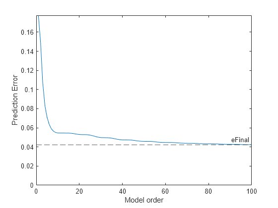
[___,eEvolution] = rlevinson(___) also returns the prediction errors from each iteration of the reverse Levinson-Durbin recursion.

example

Examples

collapse all

Optimum Autoregressive Model Order

Open Live Script

Estimate the spectrum of two sine waves in noise using an autoregressive model. Choose the best model order from a group of models returned by the reverse Levinson-Durbin recursion.

Generate a 50,000-sample signal. Specify a sample rate of 1 kHz and a signal duration of 50 seconds. The sinusoids have frequencies of 50 Hz and 55 Hz. The noise has a variance of ${(0.2)}^{2}$ .

rng default
Ns = 50e3;
Fs = 1000;
t = (0:Ns-1)'/Fs;

x = sin(2*pi*50*t) + sin(2*pi*55*t) + 0.2*randn(Ns,1);

Estimate the autoregressive model parameters using a model of order 100.

[ar,eFinal] = arcov(x,100);

Solve the model using the reverse Levinson-Durbin recursion to estimate the autocorrelation sequence, recursive prediction filters, reflection coefficients and prediction errors.

[r,u,k,eEvol] = rlevinson(ar,eFinal);

Plot the prediction errors. Add a horizontal line for the final error power. The error decreases with an increasing filter order until reaching the final error power.

plot(eEvol)
hold on
yline(eFinal,"--","eFinal")
hold off
ylim([0 eEvol(1)])
xlabel("Model order")
ylabel("Prediction Error")

Figure contains an axes object. The axes object with xlabel Model order, ylabel Prediction Error contains 2 objects of type line, constantline.

Estimate the power spectral density (PSD) for orders 1, 5, 25, 50, and 100. Estimate the PSD for the original autoregressive parameters.

N = [1 5 25 50 100];
nFFT = 8096;
psdARpred = zeros(nFFT,5);

for idx = 1:numel(N)
    order = N(idx);
    ARpred = flipud(u(:,order));
    psdARpred(:,idx) = 1./abs(fft(ARpred,nFFT)).^2;
end
psdAR = 1./abs(fft(ar,nFFT)).^2;

Plot the PSD estimates. The PSD estimates for the prediction filters get progressively closer to the original autoregressive parameters as the order increases.

F = (0:1/nFFT:1/2-1/nFFT)*Fs;

figure
plot(F,pow2db(psdARpred(1:length(psdARpred)/2,:)))
hold on
plot(F,pow2db(psdAR(1:length(psdAR)/2)),"--k")
hold off
grid

legend(["Order = "+N';"Original AR"])
xlabel("Frequency (Hz)")
ylabel("Power (dB/Hz)")
xlim([35 70])

Figure contains an axes object. The axes object with xlabel Frequency (Hz), ylabel Power (dB/Hz) contains 6 objects of type line. These objects represent Order = 1, Order = 5, Order = 25, Order = 50, Order = 100, Original AR.

Input Arguments

collapse all

`a` — Prediction filter coefficients
vector

Prediction filter coefficients, specified as a vector.

Note

The filter associated with a must be minimum phase to generate a valid autocorrelation sequence r.

If a is not minimum phase , the rlevinson function can return NaN or Inf values, even if a solution exists.

Data Types: single | double
Complex Number Support: Yes

`eFinal` — Final prediction error power
scalar

Final prediction error power, specified as a scalar.

Data Types: single | double
Complex Number Support: Yes

Output Arguments

collapse all

`r` — Autocorrelation sequence
column vector

Autocorrelation sequence, returned as a column vector with the same number of elements as in a.

`u` — Recursive prediction filter polynomial matrix
matrix

Recursive prediction filter polynomial matrix, returned as a square matrix with as many rows and columns as in the number of elements of a.

`k` — Reflection coefficients
column vector

List of reflection coefficients, returned as a column vector of length p, where p+1 is the number of elements of a.

`eEvolution` — Recursive prediction errors
row vector

List of recursive prediction errors from each iteration of the reverse Levinson-Durbin recursion, returned as a row vector. The vector eEvolution has a length p, where p+1 is the number of elements of a.

Algorithms

The reverse Levinson-Durbin recursion implements the step-down algorithm for solving the symmetric Toeplitz system of linear equations

$[\begin{matrix} r (1) & r {(2)}^{*} & \dots & r {(p - 1)}^{*} & r {(p)}^{*} \\ r (2) & r (1) & \dots & r {(p - 2)}^{*} & r {(p - 1)}^{*} \\ ⋮ & ⋮ & ⋱ & ⋮ & ⋮ \\ r (p - 1) & r (p - 2) & \dots & r (1) & r {(2)}^{*} \\ r (p) & r (p - 1) & \dots & r (2) & r (1) \end{matrix}] [\begin{matrix} a (2) \\ a (3) \\ ⋮ \\ a (p) \\ a (p + 1) \end{matrix}] = [\begin{matrix} - r (2) \\ - r (3) \\ ⋮ \\ - r (p) \\ - r (p + 1) \end{matrix}],$

where r = [r(1) r(2) … r(p) r(p + 1)] and a = [1 a(2) … a(p + 1)]. The notation ^* represents the complex conjugate transpose operation.

In linear prediction applications:

The vector r represents the autocorrelation sequence of the input to a prediction filter, where r(1) is the zero-lag element. The Toeplitz matrix R is the autocorrelation matrix.

$R = [\begin{matrix} r (1) & r {(2)}^{*} & \dots & r {(p - 1)}^{*} & r {(p)}^{*} \\ r (2) & r (1) & \dots & r {(p - 2)}^{*} & r {(p - 1)}^{*} \\ ⋮ & ⋮ & ⋱ & ⋮ & ⋮ \\ r (p - 1) & r (p - 2) & \dots & r (1) & r {(2)}^{*} \\ r (p) & r (p - 1) & \dots & r (2) & r (1) \end{matrix}]$
The vector a represents the polynomial coefficients of this prediction filter in descending powers of z.
The scalar p represents the order of the prediction filter.
$A (z) = 1 + a (2) z^{- 1} + \dots + a (n + 1) z^{- p}$

The figure shows the typical filter of this type, where H(z) is the optimal linear predictor, x(n) is the input signal, $\hat{x} (n)$ is the predicted signal, and e(n) is the prediction error signal. The variance of the prediction error, var(e) is the scalar prediction error power.

The rlevinson function solves this system of equations to compute the autocorrelation sequence r, given a vector a with the prediction filter coefficients. The filter must be minimum-phase to generate a valid autocorrelation sequence. The scalar eFinal represents the final prediction error power, var(e), and aims to be the target estimation error of the Levinson-Durbin recursion that the rlevinson function implements.

If you request the outputs u, k, or eEvolution, rlevinson also performs the UDU^* decomposition of the inverse of the autocorrelation matrix, R⁻¹. This decomposition resolves the matrices U and E, and permits the efficient evaluation of the inverse of the autocorrelation matrix, R⁻¹.

$R^{- 1} = U E^{- 1} U^{*}$

The output argument u returns the matrix U. This matrix contains the recursive prediction filter polynomials (a₁, a₂, …, a_p+1) from each iteration of the reverse Levinson-Durbin recursion.

$U = [\begin{matrix} a_{1} {(1)}^{*} & a_{2} {(2)}^{*} & \dots & a_{p + 1} {(p + 1)}^{*} \\ 0 & a_{2} {(1)}^{*} & \dots & a_{p + 1} {(p)}^{*} \\ 0 & 0 & \dots & a_{p + 1} {(p - 1)}^{*} \\ ⋮ & ⋮ & ⋱ & ⋮ \\ 0 & \dots & 0 & a_{p + 1} {(1)}^{*} \end{matrix}]$

Each vector a_i lists the recursive polynomial coefficients, where a_i(j) is the jth coefficient of the (i-1)th order prediction filter polynomial (i.e., ith step in the recursion). For example, you can get the coefficients of the 4th order prediction filter polynomial as a₅, where a5 = u(5:-1:1,5), and this vector represents the polynomial $A_{5} (z) = a_{5} (1) + a_{5} (2) z^{- 1} + ... + a_{5} (5) z^{- 4}$ . Consequently, the (p+1)th column of U contains the input polynomial coefficient vector a, which you can get using u(p+1:-1:1,p+1)'.

The output argument k returns a column vector with the reflection coefficients, which are the conjugates of the nondiagonal elements in the first row of U. In other words, k is returned as u(1,2:end)'.

$k = [\begin{matrix} a_{2} {(2)}^{*} \\ a_{3} {(3)}^{*} \\ ⋮ \\ a_{p + 1} {(p + 1)}^{*} \end{matrix}]$

The output argument eEvolution returns a row vector with the recursive prediction errors, which come from the diagonal of the matrix E, except the first element.

$E = [\begin{matrix} e_{1} & 0 & \dots & 0 \\ 0 & e_{2} & ⋱ & 0 \\ ⋮ & ⋱ & ⋱ & ⋮ \\ 0 & \dots & 0 & e_{p + 1} \end{matrix}]$

$e E v o l u t i o n = [\begin{matrix} e_{2} & e_{3} & \dots & e_{p + 1} \end{matrix}]$

Each element e_i lists the recursive prediction errors of the (i-1)th order prediction filter polynomial (i.e., ith step in the recursion). For example, you can get the prediction error of the 4th order prediction filter polynomial as e5 = eEvolution(4), and is the prediction error for using the polynomial $A_{5} (z) = a_{5} (1) + a_{5} (2) z^{- 1} + ... + a_{5} (5) z^{- 4}$ as a prediction filter.

The first element from the diagonal of E, e₁, coincides with the first element of the autocorrelation sequence r, r(1).
The (p+1)th element from the diagonal of E, e₁, —also the last element in eEvolution— coincides with the final prediction error power eFinal.

References

[1] Kay, Steven M. Modern Spectral Estimation: Theory and Application. Englewood Cliffs, NJ: Prentice-Hall, 1988.

Extended Capabilities

C/C++ Code Generation
Generate C and C++ code using MATLAB® Coder™.

Usage notes and limitations:

See Variable-Sizing Restrictions for Code Generation of Toolbox Functions (MATLAB Coder)

Version History

Introduced before R2006a

rlevinson

Syntax

Description

Examples

Optimum Autoregressive Model Order

Input Arguments

a — Prediction filter coefficients vector

eFinal — Final prediction error power scalar

Output Arguments

r — Autocorrelation sequence column vector

u — Recursive prediction filter polynomial matrix matrix

k — Reflection coefficients column vector

eEvolution — Recursive prediction errors row vector

Algorithms

References

Extended Capabilities

C/C++ Code Generation Generate C and C++ code using MATLAB® Coder™.

Version History

See Also

`a` — Prediction filter coefficients
vector

`eFinal` — Final prediction error power
scalar

`r` — Autocorrelation sequence
column vector

`u` — Recursive prediction filter polynomial matrix
matrix

`k` — Reflection coefficients
column vector

`eEvolution` — Recursive prediction errors
row vector

C/C++ Code Generation
Generate C and C++ code using MATLAB® Coder™.