Compute and Display Order-RPM Map

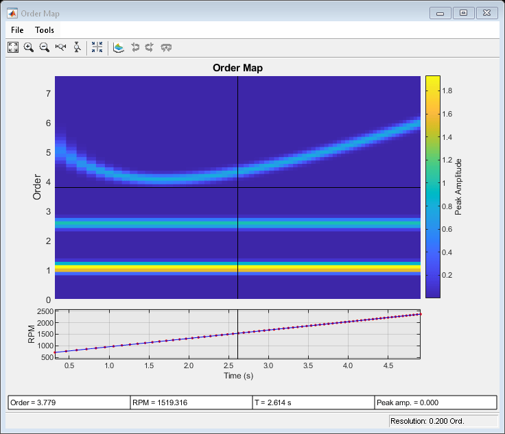
Generate a signal that consists of two linear chirps and a quadratic chirp, all sampled at 600 Hz for 5 seconds. The system that produces the signal increases its rotational speed from 10 to 40 revolutions per second during the testing period.

Generate the tachometer readings.

fs = 600;
t1 = 5;
t = 0:1/fs:t1;
f0 = 10;
f1 = 40;
rpm = 60*linspace(f0,f1,length(t));

The linear chirps have orders 1 and 2.5. The component with order 1 has twice the amplitude of the other. The quadratic chirp starts at order 6 and returns to this order at the end of the measurement. Its amplitude is 0.8. Create the signal using this information.

o1 = 1;
o2 = 2.5;
o6 = 6;
x = 2*chirp(t,o1*f0,t1,o1*f1)+chirp(t,o2*f0,t1,o2*f1) + ...
    0.8*chirp(t,o6*f0,t1,o6*f1,'quadratic');

Compute the order-RPM map of the signal. Use the peak amplitude at each measurement cell. Specify a resolution of 0.25 orders. Window the data with a Chebyshev window whose sidelobe attenuation is 50 dB.

[map,or,rp] = rpmordermap(x,fs,rpm,0.25, ...
    'Amplitude','peak','Window',{'chebwin',50});

Draw the order-RPM map as a waterfall plot.

[OR,RP] = meshgrid(or,rp);
waterfall(OR,RP,map')
view(-15,45)
xlabel('Order')
ylabel('RPM')
zlabel('Amplitude')

Use rpmordermap with no output arguments to display the map. Specify a resolution of 0.2 orders and 80% overlap between adjoining segments. Set the sidelobe attenuation of the Chebyshev window to 80 dB.

rpmordermap(x,fs,rpm,0.2, ...
    'Amplitude','peak','OverlapPercent',80,'Window',{'chebwin',80})

See Also

orderspectrum | ordertrack | orderwaveform | rpmfreqmap | rpmordermap | tachorpm