orderspectrum

Create a simulated signal sampled at 600 Hz for 5 seconds. The system that is being tested increases its rotational speed from 10 to 40 revolutions per second during the observation period.

Generate the tachometer readings.

fs = 600;
t1 = 5;
t = 0:1/fs:t1;

f0 = 10;
f1 = 40;
rpm = 60*linspace(f0,f1,length(t));

The signal consists of four harmonically related chirps with orders 1, 0.5, 4, and 6. The order-4 chirp has twice the amplitude of the others. To generate the chirps, use the trapezoidal rule to express the phase as the integral of the rotational speed.

o1 = 1;
o2 = 0.5;
o3 = 4;
o4 = 6;

ph = 2*pi*cumtrapz(rpm/60)/fs;

x = [1 1 2 1]*cos([o1 o2 o3 o4]'*ph);

Visualize the order-RPM map of the signal.

rpmordermap(x,fs,rpm)

Visualize the average order spectrum of the signal. The peaks of the spectrum correspond to the ridges seen in the order-RPM map.

orderspectrum(x,fs,rpm)

Analyze simulated data from an accelerometer placed in the cockpit of a helicopter.

Load the helicopter data. The vibrational measurements, vib, are sampled at a rate of 500 Hz for 10 seconds. The data has a linear trend. Remove the trend to prevent it from degrading the quality of the order estimation.

load('helidata.mat')

vib = detrend(vib);

Plot the nonlinear RPM profile. The rotor runs up until it reaches a maximum rotational speed of about 27,600 revolutions per minute and then coasts down.

plot(t,rpm)
xlabel('Time (s)')
ylabel('RPM')

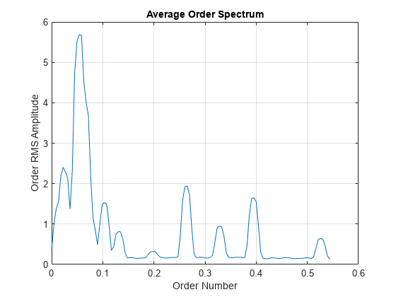
Compute the average order spectrum of the signal. Use the default order resolution.

orderspectrum(vib,fs,rpm)

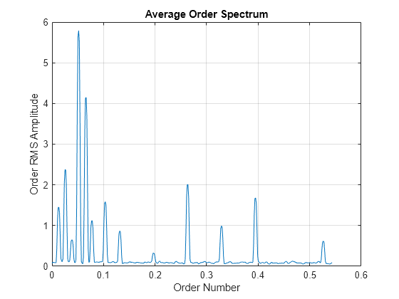
Use rpmordermap to repeat the computation with a finer order resolution. The lower orders are resolved more clearly.

[map,order] = rpmordermap(vib,fs,rpm,0.005);

orderspectrum(map,order)

Compute the power level for each estimated order. Display the result in decibels.

[map,order] = rpmordermap(vib,fs,rpm,0.005,'Amplitude','power');

spec = orderspectrum(map,order);

plot(order,pow2db(spec))
xlabel('Order Number')
ylabel('Order Power Amplitude (dB)')
grid on

References

[1] Brandt, Anders. Noise and Vibration Analysis: Signal Analysis and Experimental Procedures. Chichester, UK: John Wiley & Sons, 2011.
[2] Vold, Håvard, and Jan Leuridan. “High Resolution Order Tracking at Extreme Slew Rates Using Kalman Tracking Filters.” Shock and Vibration. Vol. 2, 1995, pp. 507–515.
Extended Capabilities
C/C++ Code Generation
Generate C and C++ code using MATLAB® Coder™.
Version History
Introduced in R2016b