Speaker Crossover Filters

Open Live Script

This example shows how to devise a simple model of a digital three-way loudspeaker. The system splits the audio input into low-, mid-, and high-frequency bands that correspond respectively to the woofer, the midrange driver, and the tweeter. Typical values for the normalized crossover frequencies that delimit the bands are $0.136 π$ rad/sample and $0.317 π$ rad/sample.

Create lowpass, bandpass, and highpass filters to generate the low-frequency, mid-frequency, and high-frequency bands. Specify the frequencies.

lo = 0.136;
hi = 0.317;

Use a 6th-order Chebyshev Type I design for each filter. Specify a passband ripple of 1 dB, larger than the value for real speakers. The cheby1 function doubles the order of bandpass designs. Make all filters have the same order by halving the order of the bandpass filter. Return the zeros, poles, and gain of each filter.

ord = 6;
rip = 1;

[zw,pw,kw] = cheby1(ord,rip,lo);
[zm,pm,km] = cheby1(ord/2,rip,[lo hi]);
[zt,pt,kt] = cheby1(ord,rip,hi,'high');

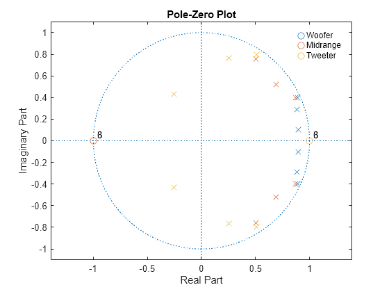
Visualize the zeros and poles of the filters.

zplane([zw zm zt],[pw pm pt])
lg = legend('Woofer','Midrange','Tweeter');
lg.Box = 'off';

Figure contains an axes object. The axes object with title Pole-Zero Plot, xlabel Real Part, ylabel Imaginary Part contains 11 objects of type line, text. One or more of the lines displays its values using only markers These objects represent Woofer, Midrange, Tweeter.

Woofer: The zeros at $z = - 1$ suppress high frequencies. The poles enhance the magnitude response between $0$ and the lower crossover frequency.
Midrange: The zeros at $z = 0$ and $z = 1$ suppress high and low frequencies. The poles enhance the magnitude response between the lower and higher crossover frequencies.
Tweeter: The zeros at $z = 1$ suppress low frequencies. The poles enhance the magnitude response between the higher crossover frequency and $π$ .

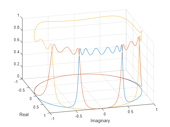
Plot the magnitude responses on the unit circle to see the effect of the different poles and zeros. Use linear units. Represent the filters as second-order sections.

sw = zp2sos(zw,pw,kw);
sm = zp2sos(zm,pm,km);
st = zp2sos(zt,pt,kt);

nf = 1024;
[hw,fw] = freqz(sw,nf,'whole');
hm = freqz(sm,nf,'whole');
ht = freqz(st,nf,'whole');

plot3(cos(fw),sin(fw),[abs(hw) abs(hm) abs(ht)])
xlabel('Real')
ylabel('Imaginary')
view(75,30)
grid

Figure contains an axes object. The axes object with xlabel Real, ylabel Imaginary contains 3 objects of type line.

Plot the magnitude responses in dB.

plot(fw/pi,mag2db(abs([hw hm ht])))
legend('Woofer','Mid-range','Tweeter')
xlabel('Normalized Frequency (\times\pi rad/sample)')
ylabel('Magnitude (dB)')
ylim([-60 0])

Figure contains an axes object. The axes object with xlabel Normalized Frequency ( times pi blank rad/sample), ylabel Magnitude (dB) contains 3 objects of type line. These objects represent Woofer, Mid-range, Tweeter.

Load an audio file containing a fragment of Handel's "Hallelujah Chorus" sampled at 8192 Hz. Split the signal into three frequency bands by filtering. Plot the bands.

load handel                % To hear, type soundsc(y,Fs)

yw = sosfilt(sw,y);        % To hear, type soundsc(yw,Fs)
ym = sosfilt(sm,y);        % To hear, type soundsc(ym,Fs)
yt = sosfilt(st,y);        % To hear, type soundsc(yt,Fs)

plot((0:length(y)-1)/Fs,[yw ym yt])
xlabel('Time (s)')

Figure contains an axes object. The axes object with xlabel Time (s) contains 3 objects of type line.

% To hear all the frequency ranges, type soundsc(yw+ym+yt,Fs)

References

Orfanidis, Sophocles J. Introduction to Signal Processing. Englewood Cliffs, NJ: Prentice Hall, 1996.

Speaker Crossover Filters

See Also