fit
Syntax
Description
fitResults = fit(problemObject)problemObject and returns the fitted results.
[
also returns simulation data fitResults,simdataI] = fit(problemObject)simdataI using the estimated parameter
values. If problemObject.FitFunction is
"sbiofitmixed", simulations use the individual parameter
estimates.
[
also returns simulation results using population parameter estimates. This syntax is
supported only when fitResults,simdataI,simdataP] = fit(problemObject)problemObject.FitFunction is
"sbiofitmixed".
Examples
This example shows how to estimate PK parameters of a SimBiology® model using a problem-based approach.
Load a synthetic data set. It contains drug plasma concentration data measured in both central and peripheral compartments.
load('data10_32R.mat')Convert the data set to a groupedData object.
gData = groupedData(data);
gData.Properties.VariableUnits = ["","hour","milligram/liter","milligram/liter"];
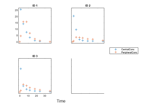
Display the data.
sbiotrellis(gData,"ID","Time",["CentralConc","PeripheralConc"],...
            Marker="+",LineStyle="none");
Use the built-in PK library to construct a two-compartment model with infusion dosing and first-order elimination. Use the configset object to turn on unit conversion.
pkmd                 = PKModelDesign;
pkc1                 = addCompartment(pkmd,"Central");
pkc1.DosingType      = "Infusion";
pkc1.EliminationType = "linear-clearance";
pkc1.HasResponseVariable = true;
pkc2                 = addCompartment(pkmd,"Peripheral");
model2cpt            = construct(pkmd);
configset            = getconfigset(model2cpt);
configset.CompileOptions.UnitConversion = true;
Assume every individual receives an infusion dose at time = 0, with a total infusion amount of 100 mg at a rate of 50 mg/hour. For details on setting up different dosing strategies, see Doses in SimBiology Models.
dose             = sbiodose("dose","TargetName","Drug_Central");
dose.StartTime   = 0;
dose.Amount      = 100;
dose.Rate        = 50;
dose.AmountUnits = "milligram";
dose.TimeUnits   = "hour";
dose.RateUnits   = "milligram/hour";
Create a problem object.
problem = fitproblem
problem =
  fitproblem with properties:

   Required:
                   Data: [0×0 groupedData]
              Estimated: [1×0 estimatedInfo]
            FitFunction: "sbiofit"
                  Model: [0×0 SimBiology.Model]
            ResponseMap: [1×0 string]

   Optional:
                  Doses: [0×0 SimBiology.Dose]
           FunctionName: "auto"
                Options: []
           ProgressPlot: 0
            UseParallel: 0
               Variants: [0×0 SimBiology.Variant]
             ErrorModel: "constant"

   sbiofit options:
                 Pooled: "auto"
    SensitivityAnalysis: "auto"
                Weights: []
Define the required properties of the object.
problem.Data        = gData;
problem.Estimated   = estimatedInfo(["log(Central)","log(Peripheral)","Q12","Cl_Central"],InitialValue=[1 1 1 1]);
problem.Model       = model2cpt;
problem.ResponseMap = ["Drug_Central = CentralConc","Drug_Peripheral = PeripheralConc"];
Define the dose to be applied during fitting.
problem.Doses = dose;
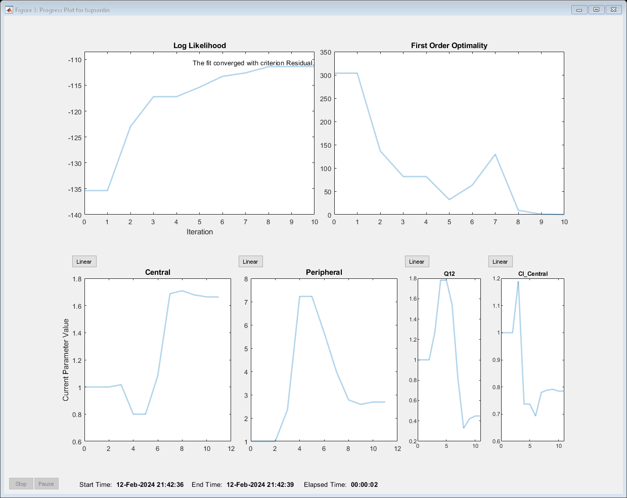
Show the progress of the estimation.
problem.ProgressPlot = true;
Fit the model to all of the data pooled together: that is, estimate one set of parameters for all individuals by setting the Pooled property to true.
problem.Pooled = true;
Perform the estimation using the fit function of the object.
pooledFit = fit(problem);
Display the estimated parameter values.
pooledFit.ParameterEstimates
ans=4×3 table
         Name         Estimate    StandardError
    ______________    ________    _____________

    {'Central'   }     1.6627        0.16569
    {'Peripheral'}     2.6864         1.0644
    {'Q12'       }    0.44945        0.19943
    {'Cl_Central'}    0.78497       0.095621
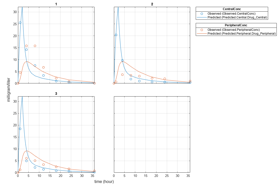
Plot the fitted results.
plot(pooledFit);
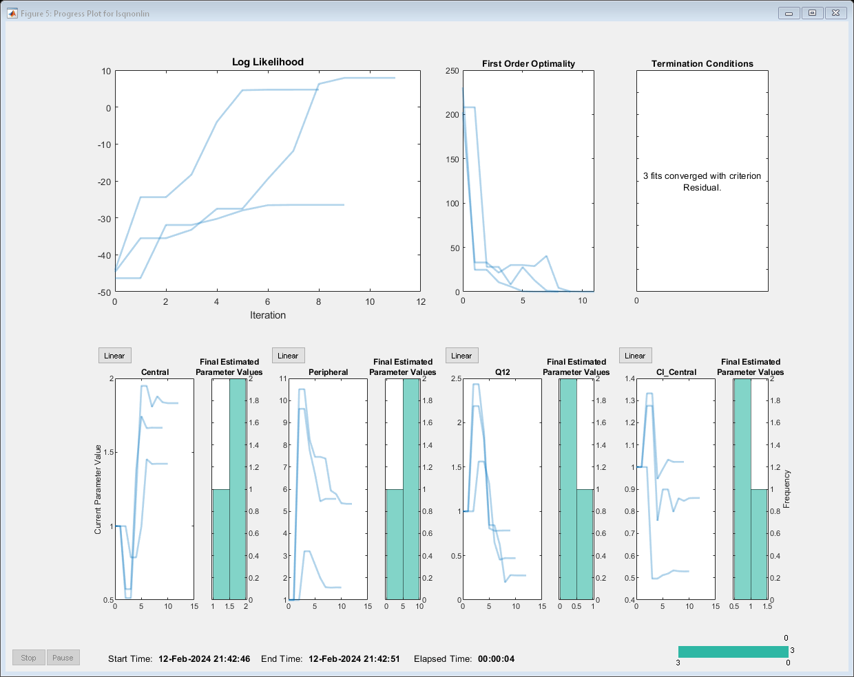
Estimate one set of parameters for each individual and see if the parameter estimates improve.
problem.Pooled  = false;
unpooledFit     = fit(problem);
Display the estimated parameter values.
unpooledFit.ParameterEstimates
ans=4×3 table
         Name         Estimate    StandardError
    ______________    ________    _____________

    {'Central'   }      1.422        0.12334
    {'Peripheral'}     1.5619        0.36355
    {'Q12'       }    0.47163        0.15196
    {'Cl_Central'}     0.5291       0.036978
ans=4×3 table
         Name         Estimate    StandardError
    ______________    ________    _____________

    {'Central'   }     1.8322       0.019672
    {'Peripheral'}     5.3364        0.65327
    {'Q12'       }     0.2764       0.030799
    {'Cl_Central'}    0.86035       0.026257
ans=4×3 table
         Name         Estimate    StandardError
    ______________    ________    _____________

    {'Central'   }     1.6657       0.038529
    {'Peripheral'}     5.5632        0.37063
    {'Q12'       }    0.78361       0.058657
    {'Cl_Central'}     1.0233       0.027311
plot(unpooledFit);
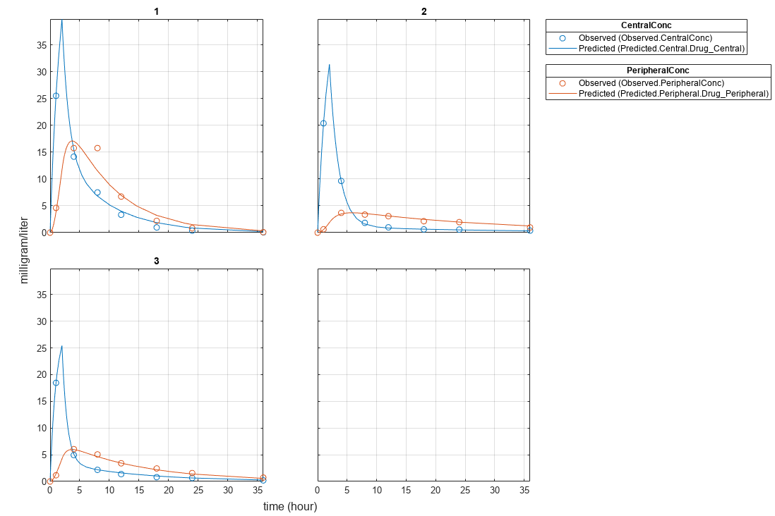
Generate a plot of the residuals over time to compare the pooled and unpooled fit results. The figure indicates unpooled fit residuals are smaller than those of the pooled fit, as expected. In addition to comparing residuals, other rigorous criteria can be used to compare the fitted results.
t = [gData.Time;gData.Time];
res_pooled = vertcat(pooledFit.R);
res_pooled = res_pooled(:);
res_unpooled = vertcat(unpooledFit.R);
res_unpooled = res_unpooled(:);
figure;
plot(t,res_pooled,"o",MarkerFaceColor="w",markerEdgeColor="b")
hold on
plot(t,res_unpooled,"o",MarkerFaceColor="b",markerEdgeColor="b")
refl = refline(0,0); % A reference line representing a zero residual
title("Residuals versus Time");
xlabel("Time");
ylabel("Residuals");
legend(["Pooled","Unpooled"]);
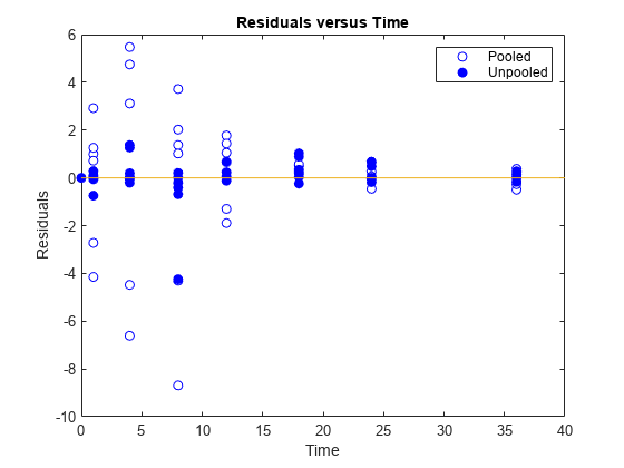
As illustrated, the unpooled fit accounts for variations due to the specific subjects in the study, and, in this case, the model fits better to the data. However, the pooled fit returns population-wide parameters. As an alternative, if you want to estimate population-wide parameters while considering individual variations, you can perform nonlinear mixed-effects (NLME) estimation by setting problem.FitFunction to sbiofitmixed.
problem.FitFunction = "sbiofitmixed";NLMEResults = fit(problem);
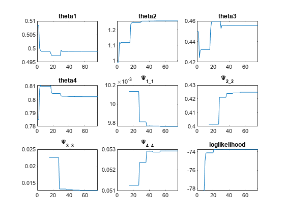
Display the estimated parameter values.
NLMEResults.IndividualParameterEstimates
ans=12×3 table
    Group         Name         Estimate
    _____    ______________    ________

      1      {'Central'   }     1.4623
      1      {'Peripheral'}     1.5306
      1      {'Q12'       }     0.4587
      1      {'Cl_Central'}    0.53208
      2      {'Central'   }      1.783
      2      {'Peripheral'}     6.6623
      2      {'Q12'       }     0.3589
      2      {'Cl_Central'}     0.8039
      3      {'Central'   }     1.7135
      3      {'Peripheral'}     4.2844
      3      {'Q12'       }    0.54895
      3      {'Cl_Central'}     1.0708
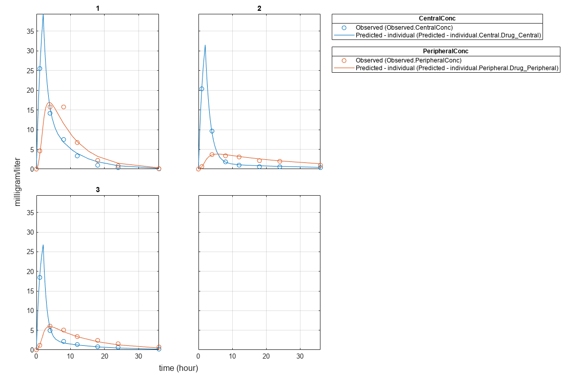
Plot the fitted results.
plot(NLMEResults);
Plot the conditional weighted residuals (CWRES) and individual weighted residuals (IWRES) of model predicted values.
plotResiduals(NLMEResults,'predictions')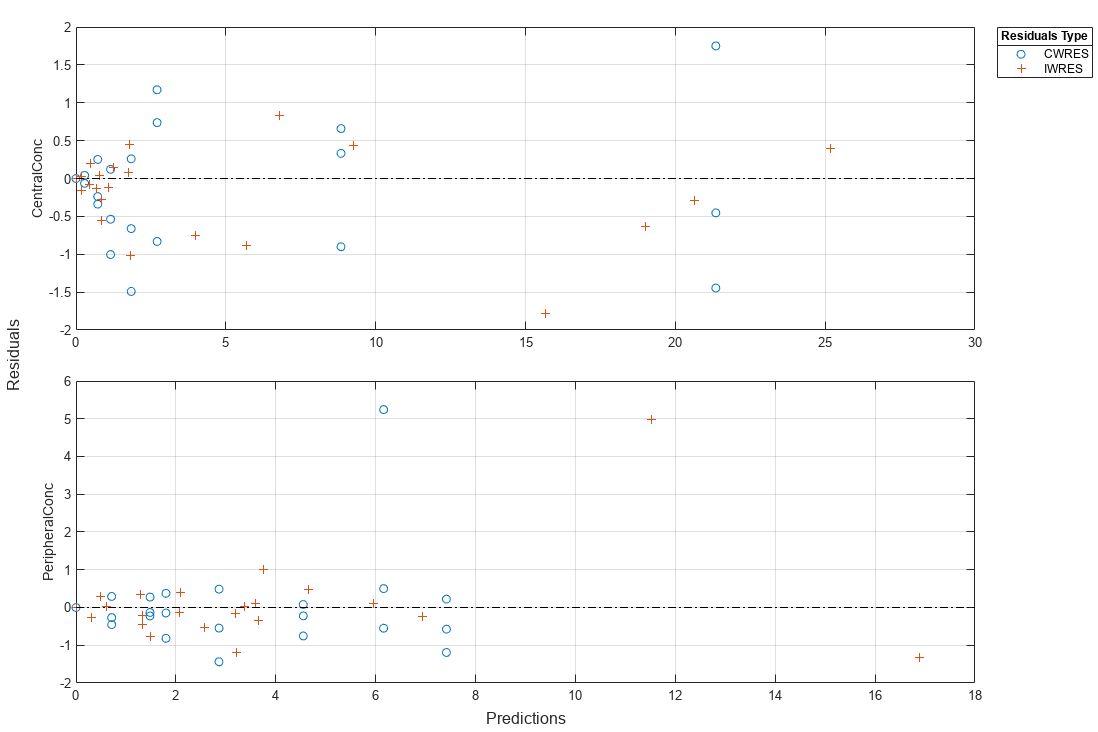
Input Arguments
SimBiology estimation problem, specified as a fitproblem
object.
Output Arguments
Estimation results, returned as a scalar OptimResults object, NLINResults object, vector of
OptimResults or NLINResults objects, or scalar
NLMEResults object.
The returned results object type varies depending on if you used
problemObject.FitFunction="sbiofit" or
problemObject.FitFunction="sbiofitmixed".
If
FitFunction="sbiofit"andFunctionName="nlinfit", the returned results object type isNLINResults. For other optimization functions, the returned object type isOptimResults.If
FitFunction="sbiofitmixed", the returned object type is alwaysNLMEResults.
When you use FitFunction="sbiofit", the function returns either a
scalar results object or vector of results objects as follows.
For an unpooled fit, the function fits each group separately using group-specific parameters,
and fitResults is a vector of results objects with one results object
for each group.
For a pooled fit, the function performs fitting for all individuals or groups simultaneously
using the same parameter estimates, and fitResults is a scalar results
object.
When the pooled option is not specified, and CategoryVariableName values of
estimatedInfo objects are all <none>,
fitResults is a single results object. This is the same behavior
as a pooled fit.
When the pooled option is not specified, and CategoryVariableName values of
estimatedInfo objects are all
<GroupVariableName>, fitResults is a
vector of results objects. This is the same behavior as an unpooled fit.
In all other cases, fitResults is a scalar object containing estimated parameter values for different groups or categories specified by CategoryVariableName.
See the Pooled property for details on how to perform a pooled, unpooled, or category fit.
When you use FitFunction="sbiofitmixed", the function always
returns a scalar NLMEResults object.
Simulation results, returned as a vector of SimData objects
representing simulation results for each group (or individual) using individual-specific
parameter estimates.
The states reported in simDataI are the states that are
included in problemObject.ResponseMap as well as any other states
listed in the StatesToLog property of the runtime
options (RuntimeOptions) of the SimBiology model
problemObject.Model.
Simulation results, returned as a vector of SimData objects
representing simulation results for each group (or individual) using only fixed-effect
estimates (population parameter estimates).
The states reported in simDataP are the states that are
included in problemObject.ResponseMap as well as any other states
listed in the StatesToLog property of the runtime
options (RuntimeOptions) of the SimBiology model
problemObject.Model.
Version History
Introduced in R2021b
See Also
MATLAB Command
You clicked a link that corresponds to this MATLAB command:
Run the command by entering it in the MATLAB Command Window. Web browsers do not support MATLAB commands.
选择网站
选择网站以获取翻译的可用内容,以及查看当地活动和优惠。根据您的位置,我们建议您选择:。
您也可以从以下列表中选择网站:
如何获得最佳网站性能
选择中国网站(中文或英文)以获得最佳网站性能。其他 MathWorks 国家/地区网站并未针对您所在位置的访问进行优化。
美洲
- América Latina (Español)
- Canada (English)
- United States (English)
欧洲
- Belgium (English)
- Denmark (English)
- Deutschland (Deutsch)
- España (Español)
- Finland (English)
- France (Français)
- Ireland (English)
- Italia (Italiano)
- Luxembourg (English)
- Netherlands (English)
- Norway (English)
- Österreich (Deutsch)
- Portugal (English)
- Sweden (English)
- Switzerland
- United Kingdom (English)