fitproblem
Description
Create a fitproblem object to estimate model parameters using
nonlinear regression or nonlinear mixed-effects modeling.
Creation
Create the object using fitproblem.
Properties
Required properties
Data to fit, specified as a groupedData
object.
The name of the time variable must be defined in the
IndependentVariableName property of Data. For
instance, if the time variable name is 'TIME', then specify it as
follows.
prob = fitproblem;
prob.Data = groupedData;
prob.Data.TIME = [1:1:10];
prob.Data.Properties.IndependentVariableName = 'TIME';
If the data contains more than one group of measurements, the grouping variable
name must be defined in the GroupVariableName property of
Data. For example, if the grouping variable name is
'GROUP', then specify it as
follows.
prob.Data.Properties.GroupVariableName = 'GROUP';Estimated parameters, specified as an estimatedInfo object, a vector of
estimatedInfo objects, or a scalar CovariateModel object.
This property defines the estimated parameters in the model and other optional
information such as their initial estimates, transformations, bound constraints, and
categories. Supported transforms are log, logit,
and probit. For details, see Parameter Transformations.
When you perform nonlinear regression by setting object.FitFunction =
"sbiofit", then:
Using
scattersearchas an optimization function requires you to specify finite transformed bounds for each estimated parameter.If you do not specify the Pooled property, the software uses the
CategoryVariableNameproperty of theestimatedInfoobject to decide if parameters must be estimated for each individual, group, category, or all individuals as a whole. Set thePooledproperty to override anyCategoryVariableNamevalues. For details about theCategoryVariableNameproperty, seeEstimatedInfo object.The software uses the
categoricalfunction to identify groups. If any group values are converted to the same value bycategorical, then those observations are treated as belonging to the same group. For instance, if some observations have no group information (that is, an empty character vector''), thencategoricalconverts empty character vectors to<undefined>, and these observations are treated as one group.
For nonlinear mixed-effects modeling with
object.FitFunction="sbiofitmixed", the
CategoryVariablename property of estimatedInfo
object is ignored.
Name of a SimBiology estimation function to use, specified as
"sbiofit" or "sbiofitmixed". Use sbiofit for nonlinear regression problems and sbiofitmixed for nonlinear mixed-effects problems.
SimBiology model used to fit the data, specified as a Model object.
Mapping between model components and data variables, specified as a character vector, string, string vector, or cell array of character vectors.
Each character vector or string is an equation-like expression, similar to
assignment rules. It contains the name (or qualified name) of a quantity (species,
compartment, or parameter) or an observable
object in the model, followed by the character '=' and the name of a
variable in Data. For clarity, white spaces are allowed between
names and '='.
For example, if you have the concentration data 'CONC' in
Data for a species 'Drug_Central', you can
specify it as
follows.
ResponseMap = 'Drug_Central = CONC';To name a species unambiguously, use the qualified name, which includes the name of the compartment. To name a reaction-scoped parameter, use the reaction name to qualify the parameter.
If the model component name or grpData variable name is not a
valid MATLAB variable name, surround it by square brackets, such as:
ResponseMap = '[Central 1].Drug = [Central 1 Conc]';If a variable name itself contains square brackets, you cannot use it in the expression to define the mapping information.
If any (qualified) name matches two components of the same type, an error is issued
when you run the fit function of the object. To resolve the error,
you can use a (qualified) name that matches two components of different types, and the
function first finds the species with the given name, followed by compartments and then
parameters.
Data Types: char | string | cell
Optional properties
Doses applied during fitting, specified as an empty array or 2-D matrix of dose
objects (ScheduleDose object or
RepeatDose object). By
default, the software applies no doses even if the model has active doses.
For a matrix of dose objects, it must have a single row or one row per group in the input data. If it has a single row, the same doses are applied to all groups during simulation. If it has multiple rows, each row is applied to a separate group, in the same order as the groups appear in the input data. Multiple columns are allowed so that you can apply multiple dose objects to each group.
For a cell vector of doses, it must have one element or one element per group in the input
data. Each element must be [] or a vector of doses. Each element of the
cell is applied to a separate group, in the same order as the groups appear in the input
data.
In addition to manually constructing dose objects using sbiodose, if the input groupedData object has dosing
information, you can use the createDoses method to construct
doses.
Name of an optimization function that is called by FitFunction
(sbiofit or sbiofitmixed), specified as a
character vector or string.
If FitFunction="sbiofit", valid choices are as follows.
"auto""fminsearch""nlinfit""fminunc"(Optimization Toolbox™ is required.)"fmincon"(Optimization Toolbox is required.)"lsqcurvefit"(Optimization Toolbox is required.)"lsqnonlin"(Optimization Toolbox is required.)"patternsearch"(Global Optimization Toolbox is required.)"ga"(Global Optimization Toolbox is required.)"particleswarm"(Global Optimization Toolbox is required.)
By default (that is, FunctionName="auto" and
FitFunction="sbiofit"), the fitproblem object uses
the first available estimation function among the following: lsqnonlin (Optimization Toolbox), nlinfit (Statistics and Machine Learning Toolbox), or fminsearch. The same priority applies to the default local solver choice
for scattersearch.
If FitFunction="sbiofitmixed", the valid choices are:
"auto""nlmefit""nlmefitsa"
When FunctionName="auto" and
FitFunction="sbiofitmixed", the object uses
"nlmefit" as the optimization function.
Data Types: char | string
Options for the optimization function, specified as a scalar struct,
optimoptions object or empty array [].
When FitFunction="sbiofit", you can use the following options:
statsetstruct fornlinfitoptimsetstruct forfminsearchoptimoptionsobject forlsqcurvefit,lsqnonlin,fmincon,fminunc,particleswarm,ga, andpatternsearchstructforscattersearch
See Default Options for Optimization Functions Called by sbiofit for more details and default options associated with each estimation function.
When FitFunction="sbiofitmixed", define a structure as follows:
The structure can contain fields and default values that are the name-value arguments accepted by
nlmefit(Statistics and Machine Learning Toolbox) andnlmefitsa(Statistics and Machine Learning Toolbox), except the following that are not supported.'FEConstDesign''FEGroupDesign’'FEObsDesign''FEParamsSelect''ParamTransform''REConstDesign''REGroupDesign''REObsDesign''Vectorization'
'REParamsSelect'is only supported when you provide a vector ofestimatedInfoobjects when specifying the estimated parameters.Use the
statset(Statistics and Machine Learning Toolbox) function only to set the'Options'field of the structure (opt), as follows.opt.Options = statset('Display','iter','TolX',1e-3,'TolFun',1e-3);
For other supported name-value arguments (see
nlmefit(Statistics and Machine Learning Toolbox) andnlmefitsa(Statistics and Machine Learning Toolbox)), set them as follows.opt.ApproximationType = 'LME';
Flag to show the progress of parameter estimation, specified as a numeric or logical
1 (true) or 0
(false). If the flag is true, a new figure opens
containing plots during fitting.
When FitFunction="sbiofit":
Plots show the log-likelihood, termination criteria, and estimated parameters for each iteration. This option is not supported for
nlinfit.If you are using the Optimization Toolbox functions (
fminunc,fmincon,lsqcurvefit,lsqnonlin), the figure also shows the First Order Optimality (Optimization Toolbox) plot.For an unpooled fit, each line on the plots represents an individual. For a pooled fit, a single line represents all individuals. The line becomes faded when the fit is complete. The plots also keep track of the progress when you run
sbiofit(for both pooled and unpooled fits) in parallel using remote clusters. For details, see Progress Plot.
When FitFunction="sbiofitmixed", the plots show the values of fixed effects parameters (theta), the estimates of the variance parameters, that is, the diagonal elements of the covariance matrix of the random effects (Ψ), and the log-likelihood. For details, see Progress Plot.
Data Types: double | logical
Flag to enable parallelization, specified as a numeric or logical
1 (true) or 0
(false). If the flag is true and Parallel Computing Toolbox™ is available, the software enables the parallelization by doing the following:
Create
SimFunctionobjects withUseParallel=true.Pass the flag
UseParallel=trueto the optimization function, such aslsqnonlin. Note that some optimization functions do not support parallelization. See the reference page of the corresponding optimization function to find out about the parallelization support.When
FitFunction="sbiofit", and you are performing an unpooled fit (Pooled=false) for multiple groups, each fit is run in parallel. For a pooled fit (Pooled=true), parallelization happens at the solver level. In other words, solver computations, such as objective function evaluations, are run in parallel.
Data Types: double | logical
Variants applied during fitting, specified as an empty array []
or a 2-D matrix or cell vector of variant objects. By default, the software applies no
variants even if the model has active variants.
For a matrix of variant objects, the number of rows must be one or must match the number of groups in the input data. The ith row of variant objects is applied to the simulation of the ith group. The variants are applied in order from the first column to the last. If this matrix has only one row of variants, they are applied to all simulations.
For a cell vector of variant objects, the number of cells must be one or must match the number
of groups in the input data. Each element must be [] or a vector
of variants. If this cell vector has a single cell containing a vector of variants,
they are applied to all simulations. If the cell vector has multiple cells, the
variants in the ith cell are applied to the simulation of the
ith group.
In addition to manually constructing variant objects using
sbiovariant, if the input groupedData
object has variant information, you can use createVariants to construct variants.
Error model used for estimation, specified as a character vector, string scalar,
string vector, cell array of character vectors, categorical vector, or table. Valid
values are "constant", "proportional",
"combined", and "exponential".
When FitFunction="sbiofit", the following applies.
If you specify only one error model, then
sbiofitestimates one set of error parameters for all responses.If you specify multiple error models using a categorical vector, string vector, or cell array of character vectors, the length of the vector or cell array must match the number of responses in
ResponseMap.You can specify multiple error models only if you are using these methods:
lsqnonlin,lsqcurvefit,fmincon,fminunc,fminsearch,patternsearch,ga, andparticleswarm. For more details, see Maximum Likelihood Estimation.If you specify weights only for the constant error model.
If you specify a table, it must contain a single variable that is a column vector of error model names. The names can be a cell array of character vectors, string vector, or a vector of categorical variables. If the table has more than one row and the
RowNamesproperty is not empty, then theRowNamesproperty must match the response variable names specified in the right hand side ofResponseMap. If the table does not use theRowNamesproperty, the nth error is associated with the nth response.
When FitFunction="sbiofitmixed", the following
applies.
You can specify only one error model.
If you specify a table, it must contain a single variable that matches one of the supported error model names.
Four built-in error models are available. Each model defines the error using a standard mean-zero and unit-variance (Gaussian) variable e, simulation results f, and one or two parameters a and b.
"constant":"proportional":"combined":"exponential":
For more details, see Error Models.
Note
If you use a
"proportional"or"combined"error model during data fitting, avoid specifying data points at times where the solution (simulation result) is zero or the steady state is zero. Otherwise, you can run into division-by-zero problems. To avoid those problems, remove those data points from the data set.For the
"exponential"error model, the software log-transforms both the input (or experimental) data and simulation results and then uses the constant error model on transformed data for parameter estimation. Consequently, fit quality metrics such as LogLikelihood, AIC, BIC, and so on are performed on log-transformed data. Hence these metrics are not directly comparable to the metrics reported for other error models.
Data Types: double | char | string | table | cell
Optional properties for FitFunction="sbiofit" only
Fit option flag to fit each individual or pool all individual data, specified as a
numeric or logical 1 (true) or
0 (false), or "auto".
If Pooled is set to "auto", the software
infers the value from the Estimated property as follows.
If Estimated is an estimatedInfo object with
its CategoryVariableName property set to the default value
<GroupVariableName>, then the Pooled
property is set to false. Otherwise, the property is set to
true.
When the property is
false, thefitfunction of the object estimates each group or individual separately using group- or individual-specific parameters, and the returned fit result is a vector of results objects with one result for each group.When the property is
true, thefitfunction performs fitting for all individuals or groups simultaneously using the same parameter estimates, and the returned result is a scalar results object.
Note
Use this option to override the CategoryVariableName value of
an estimatedInfo object.
Data Types: char | string | double | logical
Flag to use parameter sensitivities to determine gradients of the objective function, specified as a numeric or logical 1 (true) or 0 (false), or "auto".
The default behavior ("auto") is as follows.
The property is
trueforfmincon,fminunc,lsqnonlin,lsqcurvefit, andscattersearchmethods.Otherwise, the property is
false.
If it is true, the software always uses the sundials
solver, regardless of what you have selected as the SolverType property in the Configset object. If you set SensitivityAnalysis=true but
the model does not support sensitivity analysis, then the software issues an error.
The software uses the complex-step approximation method to calculate parameter sensitivities. Such calculated sensitivities can be used to determine gradients of the objective function during parameter estimation to improve fitting. The software default behavior is to first attempt to use such sensitivities to determine gradients whenever the algorithm is gradient-based and if the SimBiology model supports sensitivity analysis. If the attempt fails, the software falls back to using finite differencing to estimate gradients. For details about the model requirements and sensitivity analysis, see Sensitivity Analysis in SimBiology.
Data Types: double | logical | char | string
Weights used for fitting, specified as an empty array [], matrix of real
positive weights where the number of columns corresponds to the number of responses,
or a function handle that accepts a vector of predicted response values and returns
a vector of real positive weights.
If you specify an error model, you cannot use weights except for the constant error model. If
neither the ErrorModel or Weights is specified, by
default, the software uses the constant error model with equal weights.
Data Types: double | function_handle
Object Functions
fit | Perform parameter estimation using SimBiology problem object |
resetoptions | Reset optional SimBiology fit problem properties |
Examples
This example shows how to estimate PK parameters of a SimBiology® model using a problem-based approach.
Load a synthetic data set. It contains drug plasma concentration data measured in both central and peripheral compartments.
load('data10_32R.mat')Convert the data set to a groupedData object.
gData = groupedData(data);
gData.Properties.VariableUnits = ["","hour","milligram/liter","milligram/liter"];
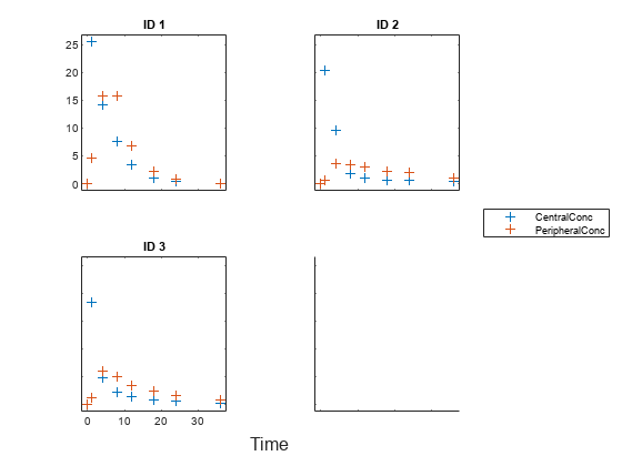
Display the data.
sbiotrellis(gData,"ID","Time",["CentralConc","PeripheralConc"],...
            Marker="+",LineStyle="none");
Use the built-in PK library to construct a two-compartment model with infusion dosing and first-order elimination. Use the configset object to turn on unit conversion.
pkmd                 = PKModelDesign;
pkc1                 = addCompartment(pkmd,"Central");
pkc1.DosingType      = "Infusion";
pkc1.EliminationType = "linear-clearance";
pkc1.HasResponseVariable = true;
pkc2                 = addCompartment(pkmd,"Peripheral");
model2cpt            = construct(pkmd);
configset            = getconfigset(model2cpt);
configset.CompileOptions.UnitConversion = true;
Assume every individual receives an infusion dose at time = 0, with a total infusion amount of 100 mg at a rate of 50 mg/hour. For details on setting up different dosing strategies, see Doses in SimBiology Models.
dose             = sbiodose("dose","TargetName","Drug_Central");
dose.StartTime   = 0;
dose.Amount      = 100;
dose.Rate        = 50;
dose.AmountUnits = "milligram";
dose.TimeUnits   = "hour";
dose.RateUnits   = "milligram/hour";
Create a problem object.
problem = fitproblem
problem =
  fitproblem with properties:

   Required:
                   Data: [0×0 groupedData]
              Estimated: [1×0 estimatedInfo]
            FitFunction: "sbiofit"
                  Model: [0×0 SimBiology.Model]
            ResponseMap: [1×0 string]

   Optional:
                  Doses: [0×0 SimBiology.Dose]
           FunctionName: "auto"
                Options: []
           ProgressPlot: 0
            UseParallel: 0
               Variants: [0×0 SimBiology.Variant]
             ErrorModel: "constant"

   sbiofit options:
                 Pooled: "auto"
    SensitivityAnalysis: "auto"
                Weights: []
Define the required properties of the object.
problem.Data        = gData;
problem.Estimated   = estimatedInfo(["log(Central)","log(Peripheral)","Q12","Cl_Central"],InitialValue=[1 1 1 1]);
problem.Model       = model2cpt;
problem.ResponseMap = ["Drug_Central = CentralConc","Drug_Peripheral = PeripheralConc"];
Define the dose to be applied during fitting.
problem.Doses = dose;
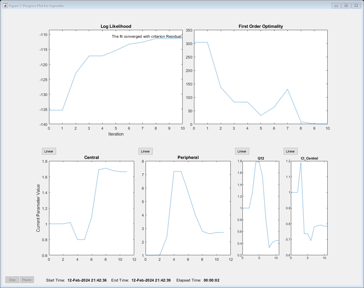
Show the progress of the estimation.
problem.ProgressPlot = true;
Fit the model to all of the data pooled together: that is, estimate one set of parameters for all individuals by setting the Pooled property to true.
problem.Pooled = true;
Perform the estimation using the fit function of the object.
pooledFit = fit(problem);
Display the estimated parameter values.
pooledFit.ParameterEstimates
ans=4×3 table
         Name         Estimate    StandardError
    ______________    ________    _____________

    {'Central'   }     1.6627        0.16569
    {'Peripheral'}     2.6864         1.0644
    {'Q12'       }    0.44945        0.19943
    {'Cl_Central'}    0.78497       0.095621
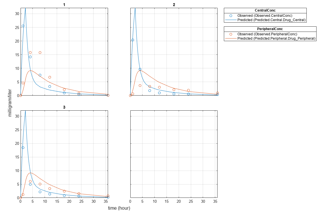
Plot the fitted results.
plot(pooledFit);
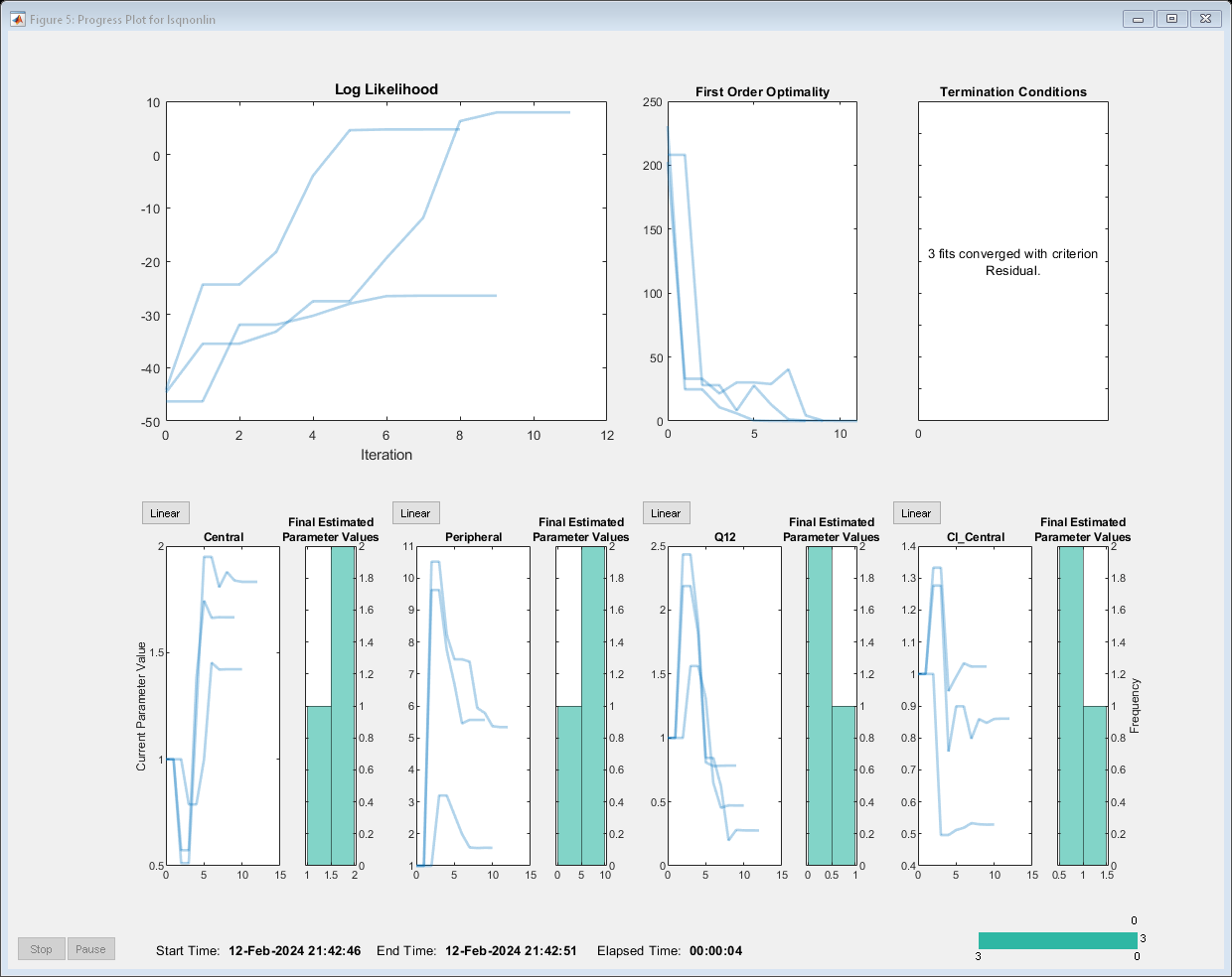
Estimate one set of parameters for each individual and see if the parameter estimates improve.
problem.Pooled  = false;
unpooledFit     = fit(problem);
Display the estimated parameter values.
unpooledFit.ParameterEstimates
ans=4×3 table
         Name         Estimate    StandardError
    ______________    ________    _____________

    {'Central'   }      1.422        0.12334
    {'Peripheral'}     1.5619        0.36355
    {'Q12'       }    0.47163        0.15196
    {'Cl_Central'}     0.5291       0.036978
ans=4×3 table
         Name         Estimate    StandardError
    ______________    ________    _____________

    {'Central'   }     1.8322       0.019672
    {'Peripheral'}     5.3364        0.65327
    {'Q12'       }     0.2764       0.030799
    {'Cl_Central'}    0.86035       0.026257
ans=4×3 table
         Name         Estimate    StandardError
    ______________    ________    _____________

    {'Central'   }     1.6657       0.038529
    {'Peripheral'}     5.5632        0.37063
    {'Q12'       }    0.78361       0.058657
    {'Cl_Central'}     1.0233       0.027311
plot(unpooledFit);
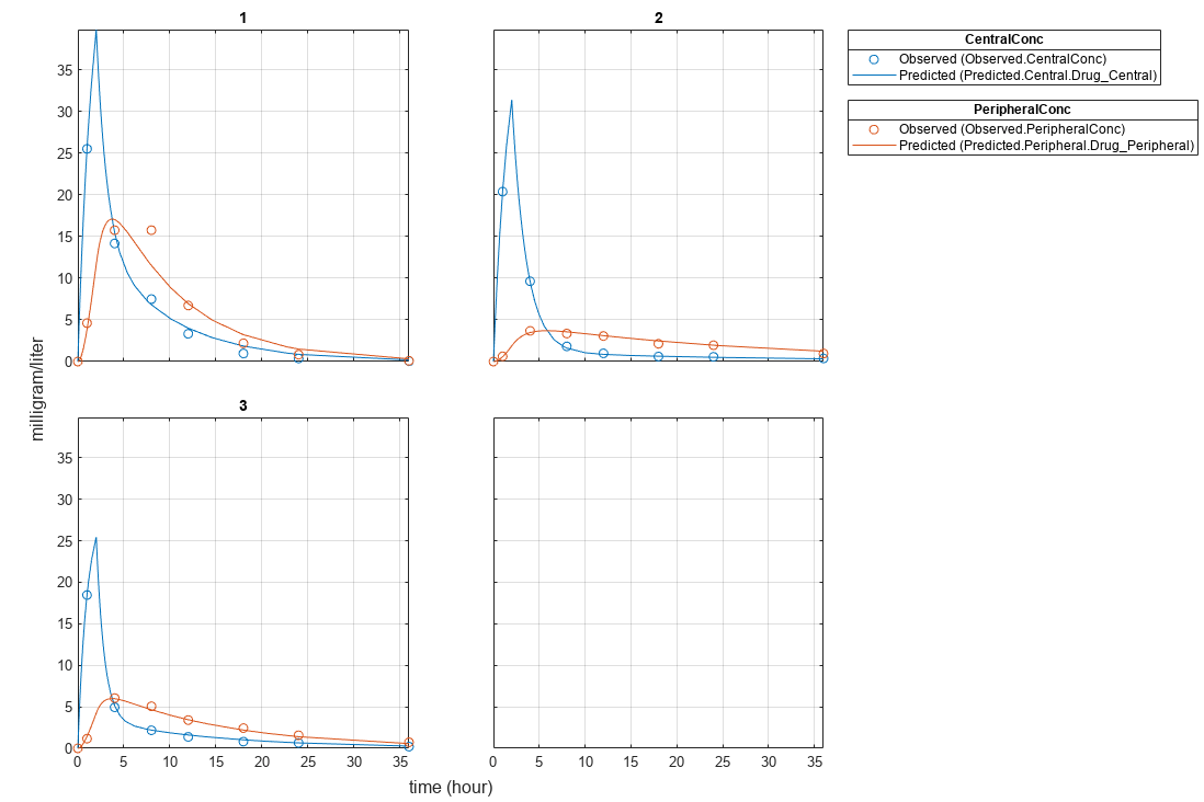
Generate a plot of the residuals over time to compare the pooled and unpooled fit results. The figure indicates unpooled fit residuals are smaller than those of the pooled fit, as expected. In addition to comparing residuals, other rigorous criteria can be used to compare the fitted results.
t = [gData.Time;gData.Time];
res_pooled = vertcat(pooledFit.R);
res_pooled = res_pooled(:);
res_unpooled = vertcat(unpooledFit.R);
res_unpooled = res_unpooled(:);
figure;
plot(t,res_pooled,"o",MarkerFaceColor="w",markerEdgeColor="b")
hold on
plot(t,res_unpooled,"o",MarkerFaceColor="b",markerEdgeColor="b")
refl = refline(0,0); % A reference line representing a zero residual
title("Residuals versus Time");
xlabel("Time");
ylabel("Residuals");
legend(["Pooled","Unpooled"]);
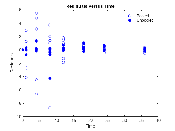
As illustrated, the unpooled fit accounts for variations due to the specific subjects in the study, and, in this case, the model fits better to the data. However, the pooled fit returns population-wide parameters. As an alternative, if you want to estimate population-wide parameters while considering individual variations, you can perform nonlinear mixed-effects (NLME) estimation by setting problem.FitFunction to sbiofitmixed.
problem.FitFunction = "sbiofitmixed";NLMEResults = fit(problem);
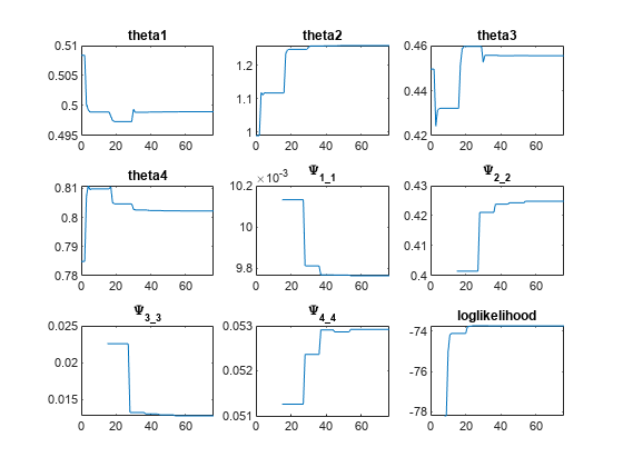
Display the estimated parameter values.
NLMEResults.IndividualParameterEstimates
ans=12×3 table
    Group         Name         Estimate
    _____    ______________    ________

      1      {'Central'   }     1.4623
      1      {'Peripheral'}     1.5306
      1      {'Q12'       }     0.4587
      1      {'Cl_Central'}    0.53208
      2      {'Central'   }      1.783
      2      {'Peripheral'}     6.6623
      2      {'Q12'       }     0.3589
      2      {'Cl_Central'}     0.8039
      3      {'Central'   }     1.7135
      3      {'Peripheral'}     4.2844
      3      {'Q12'       }    0.54895
      3      {'Cl_Central'}     1.0708
Plot the fitted results.
plot(NLMEResults);
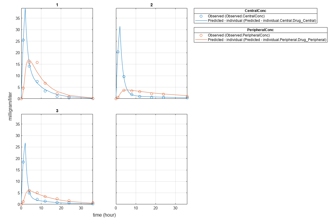
Plot the conditional weighted residuals (CWRES) and individual weighted residuals (IWRES) of model predicted values.
plotResiduals(NLMEResults,'predictions')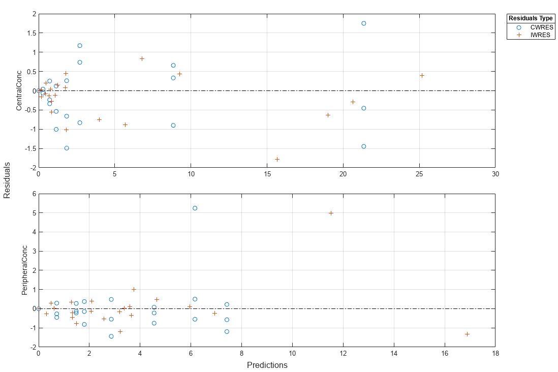
Import data to use for fitting. It comprises 12 groups of measurements across three responses: Drug, Target, and Complex. The Drug response includes measurements for all 12 groups, whereas the Target and Complex responses have measurements for only 8 and 4 groups, respectively. A group could represent a patient or an experimental or biological condition. Ndrug, Ntarget, and Ncomplex columns represent the constant number of groups that have the measurements for the corresponding responses. Each group has its own dosing amount, represented by the Dose column.
dataTMDD = readtable('tmddData_final.csv');Display the first few rows of the data set.
head(dataTMDD)
    ID    Time    Dose      Drug       Target    Complex    Ndrug    Ntarget    Ncomplex
    __    ____    ____    _________    ______    _______    _____    _______    ________

    1       0      10           NaN       NaN        NaN     12         8          4
    1     0.5     NaN        1.2131    10.116    0.36602     12         8          4
    1       1     NaN       0.74803    9.4694    0.61803     12         8          4
    1       2     NaN       0.28601    9.2434    0.84304     12         8          4
    1       4     NaN      0.048002    9.6184    0.83204     12         8          4
    1       8     NaN     0.0080003    9.6334    0.67203     12         8          4
    1      12     NaN     0.0060003    9.4574    0.54002     12         8          4
    1      16     NaN     0.0050002    9.7914    0.40502     12         8          4
Convert the data to a groupedData format.
gData = groupedData(dataTMDD);
gData.Properties.VariableUnits = ["","hour","nanomole","nanomole/liter","nanomole/liter","nanomole/liter","","",""];
gData.Properties.GroupVariableName = "ID";
gData.Properties.IndependentVariableName = "Time";
Plot the responses: Drug, Target, and Complex.
t = sbiotrellis(gData,"ID","Time","Drug",Marker="+",LineStyle="none");
plot(t,gData,"ID","Time","Target",Marker="o",LineStyle="none");
plot(t,gData,"ID","Time","Complex",Marker="^",LineStyle="none");
t.hFig.Position = [100 100 1280 800];
t.YLabel = "nanomole/liter";

Load the target-mediated drug deposition (TMDD) model. For details about the model, see Scan Dosing Regimens Using SimBiology Model Analyzer App.
sbioloadproject("tmdd_with_TO.sbproj","m1");
The data has 12 groups of measurements, and each group has its own dose amount. Create a corresponding dose object for each group using the dosing information from the data. During the subsequent fitting step, the fit function applies each dose to each group in the same order that the groups appear in the input data. For details on setting up doses, see dosing.
dose = sbiodose("Dose");
dose.TargetName = "Plasma.Drug";
doses = createDoses(gData,"Dose","",dose);
Specify parameters to estimate and their initial values. Also set upper and lower parameter bounds.
paramsToEstimate = estimatedInfo(["log(km)","log(kon)","log(koff)"],InitialValue=0.01,Bounds=[1e-05 1]);
Map the measurement data to the corresponding model components.
responseMap = ["Plasma.Drug = Drug",...
               "Plasma.Target = Target",...
               "Plasma.Complex = Complex"];
Define the algorithm options.
options                     = optimoptions("lsqnonlin");
options.StepTolerance       = 1e-08;
options.FunctionTolerance   = 1e-08;
options.OptimalityTolerance = 1e-06;
options.MaxIterations       = 100;
Define the fit problem.
f              = fitproblem(FitFunction="sbiofit");
f.Data         = gData;
f.Estimated    = paramsToEstimate;
f.Model        = m1;
f.ResponseMap  = responseMap;

f.Doses        = doses;
f.FunctionName = "lsqnonlin";
f.Options      = options;
f.Pooled       = true;
f.ProgressPlot = true;
Run the fit with weights set to 1.
f.Weights = [ones(size(gData.Drug)) ones(size(gData.Target)) ones(size(gData.Complex))];
fitEqualWeights = fit(f);

plot(fitEqualWeights);

Plot all groups in one plot for each response.
plot(fitEqualWeights,PlotStyle="one axes");
Compare the predictions to the actual data.
plotActualVersusPredicted(fitEqualWeights)

In this data set, the response Drug has 12 groups of measurements, Target has 8 groups of measurements, and Complex has 4 groups of measurements. The varying number of measurements among these responses might stem from the experimental design. To address these differences, you might consider experimenting with weights that are inversely proportional to the number of measurement groups.
f.Weights = [1./gData.Ndrug 1./gData.Ntarget 1./gData.Ncomplex];
fitInverseWeights = fit(f);

plot(fitInverseWeights);

Plot all groups in one plot for each response.
plot(fitInverseWeights,PlotStyle="one axes");
Compare the predictions to the actual data.
plotActualVersusPredicted(fitInverseWeights)

More About
The following table summarizes the default options for various estimation functions.
| Function | Default Options | ||||||
|---|---|---|---|---|---|---|---|
nlinfit (Statistics and Machine Learning Toolbox) |
| ||||||
fmincon (Optimization Toolbox) |
| ||||||
fminunc (Optimization Toolbox) |
| ||||||
fminsearch |
| ||||||
lsqcurvefit (Optimization Toolbox), lsqnonlin (Optimization Toolbox) | Requires Optimization Toolbox.
| ||||||
patternsearch (Global Optimization Toolbox) | Requires Global Optimization Toolbox.
| ||||||
ga (Global Optimization Toolbox) | Requires Global Optimization Toolbox.
| ||||||
particleswarm (Global Optimization Toolbox) | Requires Global Optimization Toolbox.
| ||||||
scattersearch | See Scatter Search Algorithm. |
Version History
Introduced in R2021b
See Also
sbiofit | sbiofitmixed | EstimatedInfo object | groupedData object | LeastSquaresResults object | NLINResults object | OptimResults object | sbiofitmixed | nlinfit (Statistics and Machine Learning Toolbox) | fmincon (Optimization Toolbox) | fminunc (Optimization Toolbox) | fminsearch | lsqcurvefit (Optimization Toolbox) | lsqnonlin (Optimization Toolbox) | patternsearch (Global Optimization Toolbox) | ga (Global Optimization Toolbox) | particleswarm (Global Optimization Toolbox)
MATLAB Command
You clicked a link that corresponds to this MATLAB command:
Run the command by entering it in the MATLAB Command Window. Web browsers do not support MATLAB commands.
选择网站
选择网站以获取翻译的可用内容,以及查看当地活动和优惠。根据您的位置,我们建议您选择:。
您也可以从以下列表中选择网站:
如何获得最佳网站性能
选择中国网站(中文或英文)以获得最佳网站性能。其他 MathWorks 国家/地区网站并未针对您所在位置的访问进行优化。
美洲
- América Latina (Español)
- Canada (English)
- United States (English)
欧洲
- Belgium (English)
- Denmark (English)
- Deutschland (Deutsch)
- España (Español)
- Finland (English)
- France (Français)
- Ireland (English)
- Italia (Italiano)
- Luxembourg (English)
- Netherlands (English)
- Norway (English)
- Österreich (Deutsch)
- Portugal (English)
- Sweden (English)
- Switzerland
- United Kingdom (English)