nlmefitsa
Fit nonlinear mixed-effects model with stochastic EM algorithm
Syntax
Description
uses the stochastic approximation expectation-maximization (SAEM) algorithm to fit the
nonlinear mixed-effects regression model beta
= nlmefitsa(X
,y
,group
,V
,modelfun
,beta0
)modelfun
to the data in
X
, y
, group
, and
V
and returns the fixed-effects estimates in
beta
. nlmefitsa
uses the initial fixed-effects
values in beta0
to fit the model.
For more information about the SAEM algorithm, see Algorithms.
Examples
Load nonlinear sample data and display the predictor, response, and grouping variables.
load nonlineardata.mat
[X,y,group]
ans = 30×5
8.1472 0.7060 75.1267 573.4851 1.0000
9.0579 0.0318 25.5095 188.3748 1.0000
1.2699 0.2769 50.5957 356.7075 1.0000
9.1338 0.0462 69.9077 499.6050 1.0000
6.3236 0.0971 89.0903 631.6939 1.0000
0.9754 0.8235 95.9291 679.1466 1.0000
2.7850 0.6948 54.7216 398.8715 1.0000
5.4688 0.3171 13.8624 109.1202 1.0000
9.5751 0.9502 14.9294 207.5047 1.0000
9.6489 0.0344 25.7508 190.7724 1.0000
1.5761 0.4387 84.0717 593.2222 1.0000
9.7059 0.3816 25.4282 203.1922 1.0000
9.5717 0.7655 81.4285 634.8833 1.0000
4.8538 0.7952 24.3525 205.9043 1.0000
8.0028 0.1869 92.9264 663.2529 1.0000
⋮
Display the group predictor variables.
V
V = 2×1
2
3
X
is a matrix of predictor data, and y
is a vector containing the response variable. group
contains data for the grouping variable, and v
contains the group predictor variables.
Create an anonymous nonlinear function that accepts a vector of coefficients, a matrix of predictor data, and a vector of group predictor variables.
model = @(phi,xfun,vfun)(phi(1).*xfun(:,1).*exp(phi(2).*xfun(:,2)./vfun)+phi(3).*xfun(:,3))
model = function_handle with value:
@(phi,xfun,vfun)(phi(1).*xfun(:,1).*exp(phi(2).*xfun(:,2)./vfun)+phi(3).*xfun(:,3))
model
is a handle for a function given by the formula
.
Fit model
to the data in X
, y
, group
, and v
using the nlmefitsa
function. Specify a vector of ones as the initial estimate for the fixed-effects coefficients.
beta = nlmefitsa(X,y,group,V,model,[1 1 1])
beta = 3×1
1.0008
4.9980
6.9999
The output shows the progress of estimating the fixed effects and the elements of the random-effects covariance matrix, as well as the final fixed-effects estimates beta
. In each plot, the horizontal axis shows the iteration step, and the vertical axis shows the value of the estimation.
Load some nonlinear sample data.
load nonlineardata.mat;
X
is a matrix of predictor data and y
is a vector containing the response variable. group
and V, respectively contain data for a grouping variable and group predictor.
Create an anonymous nonlinear function that accepts a vector of coefficients, a matrix of predictor data, and a vector of group predictor data.
model = @(phi,xfun,vfun)(phi(1).*xfun(:,1).*exp(phi(2).*xfun(:,2)./vfun)+phi(3).*xfun(:,3));
model
is a handle for a function given by the formula .
Define an output function for nlmefitsa
. For more information about the form of the output function, see the OutputFcn
field description for the Options
name-value argument.
function stop = outputFunction(beta,status,state) stop = 0; hold on plot3(status.iteration,beta(2),beta(1),"mo") state = string(state); if state=="done" stop=1; end end
outputFunction
is a function that plots the iteration number for the fitting algorithm together with the first and second fixed effects. outputFunction
returns 1
when the fitting algorithm has completed its final iteration.
Use the statset
function to create an options structure for nlmefitsa
that uses outputFunction
as its output function.
default_opts=statset("nlmefitsa");
opts = statset(default_opts,OutputFcn=@outputFunction);
opts
is a statistics options structure that contains options for the stochastic expectation maximization fitting algorithm.
Create a figure and define axes for outputFunction
to plot into. Fit model to the predictor data in X
and the response data in y
using the options in opts
.
figure ax = axes(view=[12,10]); xlabel("Iteration") ylabel("beta(2)") zlabel("beta(1)") box on [beta,psi,stats] = nlmefitsa(X,y,group,V,model,[1 1 1],Options=opts)
beta = 3×1
1.0008
4.9980
6.9999
psi = 3×3
10-4 ×
0.0415 0 0
0 0.2912 0
0 0 0.0004
stats = struct with fields:
logl: []
aic: []
bic: []
sebeta: []
dfe: 23
covb: []
errorparam: 0.0139
rmse: 0.0012
ires: [30×1 double]
pres: [30×1 double]
iwres: [30×1 double]
pwres: [30×1 double]
cwres: [30×1 double]
nlmefitsa
calls outputFunction
after every iteration of the fitting algorithm. The figure shows that the fixed effects beta(1)
and beta(2)
are near 1
when the iteration number is near 0
. This is consistent with the initial values for beta
. As the iteration number increases, beta(1)
makes a large jump up to around 3.3
before converging to 1
. As beta(1)
converges to 1
, beta(2)
converges to 5
. The output argument beta
contains the final values for the fixed effects. psi
and stats
, respectively, contain the covariance matrix for the random effects and additional statistics about the fit.
Load the indomethacin
data set.
load indomethacin
The variables time
, concentration
, and subject
contain time series data for the blood concentration of the drug indomethacin in six patients.
Create an anonymous nonlinear function that accepts a vector of coefficients and a vector of predictor variables.
model = @(phi,t)(phi(1).*exp(-phi(2).*t)+phi(3).*exp(-phi(4).*t));
model
is a handle for a function given by the formula
,
where is the concentration of indomethacin, for are coefficients, and is time. The function does not contain group-specific predictor variables because the formula does not include them.
Fit the model to the data using time
as the predictor variable, subject
as the grouping variable, and concentration
as the response. Specify a log transformation function for the second and fourth coefficients.
phi0 = [1 1 1 1];
xform = [0 1 0 1];
[beta,psi,stats,b] = nlmefitsa(time,concentration, ...
subject,[],model,phi0,ParamTransform=xform)
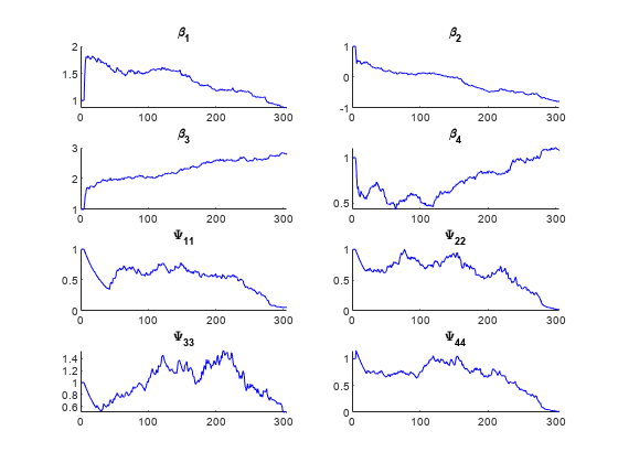
beta = 4×1
0.8630
-0.7897
2.7762
1.0785
psi = 4×4
0.0585 0 0 0
0 0.0248 0 0
0 0 0.5068 0
0 0 0 0.0139
stats = struct with fields:
logl: []
aic: []
bic: []
sebeta: []
dfe: 57
covb: []
errorparam: 0.0811
rmse: 0.0772
ires: [66×1 double]
pres: [66×1 double]
iwres: [66×1 double]
pwres: [66×1 double]
cwres: [66×1 double]
b = 4×6
-0.2302 -0.0033 0.1625 0.1774 -0.3334 0.1129
0.0363 -0.1502 0.0071 0.0471 0.0068 -0.0481
-0.7631 -0.0553 0.8780 -0.8120 0.5429 0.1695
-0.0030 -0.0223 0.0192 -0.0830 0.0505 -0.0066
The output argument beta
contains the fixed effects for the model, and b
contains the random effects. The plots show the progress of the Monte Carlo simulation used to fit the coefficients. The maximum likelihood estimates for beta
and the random-effects covariance matrix psi
converge after about 300 iterations.
Plot the sample data together with the model, using only the fixed effects in beta
for the model coefficients. Use the gscatter
function to color code the data according to the subject. To reverse the log transformation on the second and fourth coefficients, take their exponentials using the exp
function.
figure hold on gscatter(time,concentration,subject); phi = [beta(1),exp(beta(2)),beta(3),exp(beta(4))]; tt = linspace(0,8); cc = model(phi,tt); plot(tt,cc,LineWidth=2,Color="k") legend("Subject 1","Subject 2","Subject 3",... "Subject 4","Subject 5","Subject 6","Fitted curve") xlabel("Time (hours)") ylabel("Concentration (mcg/ml)") title("Indomethacin Elimination") hold off
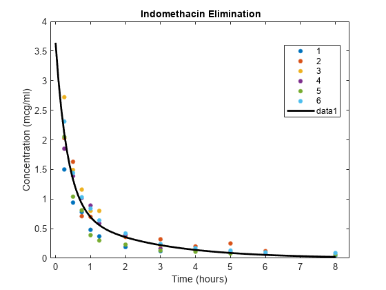
The plot shows that the blood concentration of indomethacin decreases over eight hours, and the fitted model passes through the bulk of the data.
Plot the data together with the model again, using both the fixed effects and the random effects in b
for the model coefficients. For each subject, plot the data and the fitted curve in the same color.
figure hold on h = gscatter(time,concentration,subject); for j=1:6 phir = [beta(1)+b(1,j),exp(beta(2)+b(2,j)), ... beta(3)+b(3,j),exp(beta(4)+b(4,j))]; ccr = model(phir,tt); col = h(j).Color; plot(tt,ccr,Color=col) end legend("Subject 1","Subject 2","Subject 3",... "Subject 4","Subject 5","Subject 6",... "Fitted curve 1","Fitted curve 2","Fitted curve 3",... "Fitted curve 4","Fitted curve 5","Fitted curve 6") xlabel("Time (hours)") ylabel("Concentration (mcg/ml)") title("Indomethacin Elimination") hold off
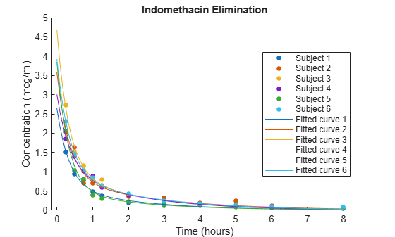
The plot shows that, for each subject, the fitted curve follows the bulk of the data more closely than the curve for the fixed-effects model in the previous figure. This result suggests that the random effects improve the fit of the model.
Input Arguments
Predictor variables, specified as an n-by-h numeric matrix, where n is the number of observations and h is the number of predictor variables.
Data Types: single
| double
Response variable, specified as a numeric vector with n elements, where n is the number of observations.
Data Types: single
| double
Grouping variable, specified as a numeric, categorical, or string vector, or a cell array of character vectors.
Example: ["subject1" "subject4" "subject3"…"subject3" "subject2"]
Example: [ones(50,1);2*ones(50,1);3*ones(50,1)]
Data Types: double
| single
| string
| cell
| categorical
Group predictor variables, specified as a numeric matrix or cell array. Group predictor variables are variables that have the same value for all observations in a group.
If the group-specific predictor variables are the same size across groups, specify
V
as an m-by-g matrix, where m is the number of groups and g is the number of group predictor variables.If the group-specific predictor variables vary in size across groups, specify
V
as an m-by-g cell array.If you do not have group predictor variables, specify
V
as[]
.
Example: [1 2; 2 4; 5 2; 7 1; 4 5; 3 6]
Data Types: single
| double
| cell
Model function, specified as a function handle. If
V
is empty, the function can have the form yfit =
modelfun(phi,xfun)
. Otherwise, it must have the form yfit =
modelfun(phi,xfun,vfun)
.
Argument | Description |
---|---|
phi |
An array of model coefficients. The size of
|
xfun |
An array of predictor variables. The size of
|
vfun |
An array of group predictor variables. The size of
If |
yfit | Fitted response values. yfit contains an element for each row in
xfun . |
For improved performance, allow modelfun
to accept predictor
variables for multiple observations and specify the Vectorization
name-value
argument as "SingleGroup"
or "Full"
.
Example: model =
@(phi,xfun,vfun)(phi(:,1).*exp(vfun(:,1).*xfun(:,1))+log(phi(:,2).*xfun(:,2)./vfun(:,1)));
beta = nlmefitsa(X,y,group,V,model,[1 1 1]);
Data Types: function_handle
Initial fixed-effects values, specified as a numeric vector or matrix.
If
beta0
is a vector, its size must be equal to the number of fixed effects.If
beta0
is a matrix, it must have as many rows as the number of model coefficients. For each column inbeta0
,nlmefitsa
repeats the estimation of the fixed effects using the column entries as the initial fixed-effects values.
Example: [1 1 1 1]
Data Types: single
| double
Name-Value Arguments
Specify optional pairs of arguments as
Name1=Value1,...,NameN=ValueN
, where Name
is
the argument name and Value
is the corresponding value.
Name-value arguments must appear after other arguments, but the order of the
pairs does not matter.
Example: nlmefitsa(X,y,group,V,model,[1 1
1],Replicates=2,Vectorization="SingleGroup")
specifies to estimate the model
function parameters twice using the same starting point, and to pass the sample data to the
model function in batches corresponding to each group.
Fixed and Random Effects
Fixed-effects coefficients, specified as a numeric or logical vector. This argument indicates which coefficients in the model function input argument phi
contain a fixed effect. For more information about the model function, see modelfun
. By default, all the elements of phi
contain fixed effects.
When you specify FEParamsSelect
, you cannot specify
FEConstDesign
or FEGroupDesign
.
Example: FEParamsSelect=[1 0 1 1]
Data Types: single
| double
| logical
Fixed-effects
design matrix, specified as a p-by-f design matrix.
p is the number of coefficients in the model function input argument
phi
, and f is the number of fixed effects. For more
information, see modelfun
and Mixed-Effects Model Hierarchy.
When you specify FEConstDesign
, you cannot specify
FEParamsSelect
or FEGroupDesign
.
Example: FEConstDesign=[0.1 0.5; 3 0.7; 0.8 2; 4 8]
specifies a
design matrix for four model parameters and two fixed effects.
Data Types: single
| double
Fixed-effects group design matrices, specified as a
p-by-f-by-m array of design
matrices. p is the number of coefficients in the model function input
argument PHI
, f is the number of fixed effects, and
m is the number of groups specified by group
.
FEGroupDesign
specifies a different
p-by-f design matrix for each of the
m groups.
When you specify FEGroupDesign
, you cannot specify
FEConstDesign
or FEParamsSelect
.
Example: A(:,:,1) = [0.1 0.5; 3 0.7; 0.8 2]; A(:,:,2) =
ones(3,2);
FEGroupDesign=A
specifies a design matrix for three model
parameters, two fixed effects, and two groups.
Data Types: single
| double
Random-effects coefficients, specified as a numeric or
logical vector. This argument indicates which coefficients in the model function input argument
PHI
contain a random effect. For more information about the model
function, see modelfun
. By default, all the elements of
PHI
contain random effects.
When you specify REParamsSelect
, you cannot specify
REConstDesign
.
Example: REParamsSelect=[0 0 1 1]
Data Types: single
| double
| logical
Random-effects design matrix, specified as a p-by-r
design matrix. p is the number of coefficients in the model function input
argument phi
, and r is the number of random effects. For
more information, see modelfun
and Mixed-Effects Model Hierarchy.
When you specify REConstDesign
, you cannot specify
REParamsSelect
.
Example: REConstDesign=[1 0 2 1; 3 1 0 0; 0 0 1 0]
specifies a
design matrix for three parameters and four random effects.
Data Types: single
| double
Iterative Algorithm
Size of the model function inputs, specified as a string scalar or character vector
with one of the following values. For more information about the model function inputs,
see modelfun
.
Value | Description |
---|---|
"SinglePhi" |
The
model function calculates |
"SingleGroup" |
The model function calculates
|
"Full" |
The model function calculates
|
If V
is an empty array,
nlmefitsa
calls the model function with two inputs.
Example: Vectorization="SingleGroup"
Data Types: string
| char
Random-effects covariance matrix pattern, specified as an
r-by-r identity, numeric, or logical matrix,
or a 1-by-r vector of integers, where r is the
number of random effects. nlmefitsa
calculates variance and
covariance estimates for the random effects specified by
CovPattern
. For more information, see
psi
.
When
CovPattern
is a matrix, each off-diagonal element corresponds to a pair of random effects, and each element along the diagonal corresponds to the variance for a single random effect.nlmefitsa
calculates variance and covariance estimates for the random effects corresponding to the nonzero elements ofCovPattern
. Zero elements inCovPattern
indicate that the variances and covariances are constrained to zero.If
CovPattern
is not a row-column permutation of a block diagonal matrix,nlmefitsa
automatically adds nonzero elements to produce such a pattern.When
CovPattern
is a vector, elements with equal values define groups of random effects. In addition to variances,nlmefitsa
calculates covariance estimates for pairs of random effects within groups, and constrains covariances across groups to zero.
The default value for CovPattern
is an
r-by-r identity matrix, which corresponds to
uncorrelated random effects.
Example: CovPattern=ones(3)
Example: CovPattern=[1 1 2]
Data Types: single
| double
| logical
Initial covariance values, specified as an r-by-r
positive definite matrix, where r is the number of random effects. A
positive definite matrix is symmetric with all nonnegative
eigenvalues. If you do not specify Cov0
,
nlmefitsa
calculates Cov0
using
beta0
.
Example: Cov0=[4 1 2; 1 2 0; 2 0 3]
Data Types: single
| double
Flag to calculate standard errors, specified as a numeric or logical 0
(false
) or 1
(true
). nlmefitsa
returns the standard errors in the stats
output argument.
Example: ComputeStdErrors=true
Data Types: single
| double
| logical
Model for the error term, specified as a string scalar or character vector containing the
model name. nlmefitsa
stores the parameter values for the error
model in the errorparam
field of the stats
output argument.
Model Name | Formula | stats.errorparam |
---|---|---|
"constant" |
| a |
"proportional" |
| b |
"combined" |
| [a,b] |
"exponential" |
| a |
In the above table, is the response variable y
, is the fitted model, and and are model parameters.
Example: ErrorModel="exponential"
Data Types: string
| char
Initial parameters for the error model, specified as a numeric scalar, 1-by-2 numeric vector, or 2-by-1 numeric vector.
If ErrorModel
is "combined"
, ErrorParameters
must be a two-element vector. Otherwise, ErrorParameters
must be a scalar.
Example: ErrorParameters=0.75
Example: ErrorParameters=[0.3,0.5]
Data Types: single
| double
Loglikelihood approximation method, specified as a string scalar or character vector containing one of the following values.
Value | Description |
---|---|
"none" | Omit the loglikelihood approximation. |
"is" | Importance sampling |
"gq" | Gaussian quadrature |
"lin" | Linearization |
Example: LogLikMethod="lin"
Data Types: string
| char
Number of burn-in iterations for the Markov chain Monte Carlo (MCMC) algorithm, specified as a
nonnegative integer. nlmefitsa
uses the
MCMC algorithm during fitting to update the expected value of
the loglikelihood function. During the burn-in iterations,
nlmefitsa
does not
recalculate the parameter estimates for the loglikelihood
function.
For more information about the nlmefitsa
fitting algorithm, see Algorithms.
Example: NBurnIn=10
Data Types: single
| double
Number of chains nlmefitsa
simulates for each iteration of the fitting
algorithm, specified as a positive integer. During an iteration,
nlmefitsa
calculates NChains
coefficient
vectors for each group. If you do not specify NChains
, the function
calculates a value that results in approximately 100 groups across all chains.
For more information about the nlmefitsa
fitting algorithm, see Algorithms.
Example: NChains=5
Data Types: single
| double
Number of iterations for each phase of the fitting algorithm, specified as a positive integer
scalar, a 1-by-3 vector of positive integers, or a 3-by-1 vector of positive integers.
NIterations
determines the number of iterations for the following:
Simulated annealing in the first step
Full step size calculation in the second step
Reduced step size calculation in the third step
When NIterations
is a vector, each element contains
the number of iterations for the step corresponding to its index. When
NIterations
is a scalar, nlmefitsa
distributes the iterations across the three phases of the fitting algorithm in the same
proportions as the default.
For more information about the nlmefitsa
fitting algorithm, see Algorithms.
Example: NIterations=500
Data Types: single
| double
Number of Markov chain Monte Carlo (MCMC) iterations in each simulation step of the fitting
algorithm, specified as a positive integer scalar, a 1-by-3 vector of positive integers,
or a 3-by-1 vector of positive integers. NMCMCIterations
determines
the number of iterations for the following:
Full multivariate update in the first step
Single coordinate update in the second step
Multiple coordinate update in the third step
When NMCMCIterations
is a vector, each element
contains the number of iterations for the step corresponding to its index. When
NMCMCIterations
is a scalar, nlmefitsa
expands the scalar to a three-element vector with elements equal to the scalar.
For more information about the nlmefitsa
fitting algorithm, see Algorithms.
Example: NMCMCIterations=[5,2,4]
Data Types: single
| double
Optimization function for maximizing the likelihood function, specified as "fminsearch"
or "fminunc"
.
"fminsearch"
— Uses a direct search method involving function evaluations only. For more information, seefminsearch
."fminunc"
— Uses gradient methods. This option, which requires Optimization Toolbox, is generally more efficient. For more information, seefminunc
(Optimization Toolbox).
For more information about the nlmefitsa
fitting algorithm, see Algorithms.
Example: OptimFun="fminunc"
Data Types: string
| char
Options,
specified as a statistics options structure returned by the statset
function. The structure contains the following fields.
Field | Description |
---|---|
DerivStep |
Relative difference used in the finite difference gradient
calculation, specified as a positive scalar, or as a vector of the same
length as the |
Display |
Option to display algorithm information, specified as one of the following:
|
FunValCheck |
Flag to check for invalid values returned by the model function, specified as one of the following.
|
OutputFcn |
Output function, specified as a function handle or a cell array of
function handles.
The default output function plots the progress of the fitting algorithm for estimating the fixed effects, and plots the random-effects variances. |
Streams | Streams used by nlmefitsa when generating random
numbers, specified as a RandStream object. The default
is the current global stream. |
TolX | Termination tolerance for the fixed- and random-effects estimates. The
default is 1e-4 . |
Example: Options=statset("nlmefitsa")
Data Types: struct
Coefficient transformation function for the model function, specified as a vector of integers between 0 and 3, inclusive. ParamTransform
must have the same number of elements as the model function input argument PHI
. For more information about the model function, see modelfun
.
The coefficients for the model function are given by
where and are the original and transformed model coefficients, respectively. and are the design matrices for the fixed and random effects and , respectively. The value of ParamTransform
indicates the form of the transformation function according to the following scheme.
Value | Function |
---|---|
0 |
|
1 |
|
2 |
|
3 |
|
For more information about the fixed-effects design matrix, see
FEConstDesign
and FEGroupDesign
. For more
information about the random-effects design matrix, see
REConstDesign
.
Example: ParamTransform=[0 1 0]
Data Types: single
| double
Number of estimates for the fixed and random effects, specified as a positive integer.
When
beta0
is a vector,nlmefitsa
estimates the fixed and random effectsReplicates
number of times using the initial values inbeta0
. In this case, the default value forReplicates
is1
.When
beta0
is a matrix,nlmefitsa
estimates the fixed- and random-effects for each column inbeta0
. In this case,Replicates
must be equal to the number of columns inbeta0
.
Example: Replicates=3
Data Types: single
| double
Output Arguments
Fixed-effects coefficient estimates, returned as a numeric vector or an
f-by-k matrix. f is the
number of fixed effects and k is the number of estimates specified by
Replicates
.
Data Types: single
| double
Random-effects covariance matrices, returned as an
r-by-r numeric matrix or an
r-by-r-by-k array of
numeric matrices. r is the number of random effects and
k is the number of estimates specified by
Replicates
.
Data Types: single
| double
Fitting information, returned as a structure with the following fields.
Field | Description |
---|---|
logl | Maximized loglikelihood for the fitted model. This field is empty
if the LogLikMethod name-value argument is
"none" during fitting. |
rmse | Square root of the estimated error variance.
nlmefitsa calculates
rmse on the log scale when the
ErrorModel name-value argument is
"exponential" during fitting. |
errorparam | Estimated parameters of the error model specified by the
ErrorModel name-value argument during
fitting. |
aic | Akaike information criterion (AIC). This field is empty if the
LogLikMethod is name-value argument is
"none" during fitting.
nlmefitsa calculates the AIC as aic =
-2*logl+2*numParam , where logl is the maximized
loglikelihood for the fitted model, and numParam
is the number of fitting parameters. The fitting parameters include
the degrees of freedom for the random-effects covariance matrix, the
number of fixed effects, and the number of parameters in the error
model. |
bic | Bayesian information criterion (BIC).
This field is empty if the
|
sebeta | Standard errors for the fixed-effects estimates in
beta . This field is empty if the
ComputeStdErrors name-value argument is
false during fitting. |
covb | Estimated covariance matrix for the fixed-effects estimates
in |
dfe | Error degrees of freedom |
pres | Population residuals, given by |
ires | Individual residuals, given by |
pwres | Population weighted residuals |
cwres | Conditional weighted residuals |
iwres | Individual weighted residuals |
Data Types: struct
Random-effects estimates, returned as an r-by-m
numeric matrix or an
r-by-m-by-k array of
numeric matrices. r is the number of random effects,
m is the number of groups specified by
group
, and k is the number of replicates
specified by Replicates
.
Data Types: single
| double
Algorithms
By default, nlmefitsa
fits a model where each model coefficient is
the sum of a fixed effect and a random effect. To fit a model with a different number of fixed
and random effects, use the name-value arguments in the Fixed and Random Effects section.
To estimate the parameters of a nonlinear mixed-effects model,
nlmefitsa
uses an iterative algorithm that includes a random Monte
Carlo simulation. To specify parameters for the iterative algorithm, use the name-value
arguments in the Iterative Algorithm section. Examine the plot of
simulation results to ensure that the simulation has converged. You can also compare the
results of calling nlmefitsa
multiple times with different starting
values, or use the Replicates
name-value argument to perform multiple
simulations.
During fitting, nlmefitsa
calculates maximum likelihood
estimates, which are parameter values that maximize a likelihood function.
nlmefitsa
uses the following likelihood function:
where
is the response data.
is the vector of population coefficients.
is the residual variance.
is the covariance matrix for the random effects.
is the set of unobserved random effects.
Each pdf on the right side of the formula is a normal (Gaussian) likelihood function that might depend on covariates.
nlmefitsa
uses the stochastic approximation
expectation-maximization (SAEM) algorithm to calculate the maximum likelihood estimates [1]. The SAEM algorithm takes
these steps:
Simulation — Use a Markov chain Monte Carlo algorithm together with the posterior density function and the current parameter estimates to simulate values for . Calculate the loglikelihood for each simulated , and then take the average of the loglikelihoods.
Stochastic approximation — Update the expected value of the loglikelihood function by moving its current value toward the average calculated in the previous step.
Maximization — Choose new estimates for , , and that maximize the loglikelihood function given the simulated values of the random effects.
References
[1] Delyon, B., M. Lavielle, and E. Moulines. "Convergence of a Stochastic Approximation Version of the EM Algorithm." Annals of Statistics, 27, 94–128, 1999.
[2] Mentré, F., and M. Lavielle. "Stochastic EM Algorithms in Population PKPD Analyses." American Conference on Pharmacometrics, 2008.
Version History
Introduced in R2010a
MATLAB Command
You clicked a link that corresponds to this MATLAB command:
Run the command by entering it in the MATLAB Command Window. Web browsers do not support MATLAB commands.
Select a Web Site
Choose a web site to get translated content where available and see local events and offers. Based on your location, we recommend that you select: .
You can also select a web site from the following list
How to Get Best Site Performance
Select the China site (in Chinese or English) for best site performance. Other MathWorks country sites are not optimized for visits from your location.
Americas
- América Latina (Español)
- Canada (English)
- United States (English)
Europe
- Belgium (English)
- Denmark (English)
- Deutschland (Deutsch)
- España (Español)
- Finland (English)
- France (Français)
- Ireland (English)
- Italia (Italiano)
- Luxembourg (English)
- Netherlands (English)
- Norway (English)
- Österreich (Deutsch)
- Portugal (English)
- Sweden (English)
- Switzerland
- United Kingdom (English)