Reduce Fast Dynamics in a Linear Model
Linearize the Model
The model in this example is not linear. Before performing the frequency-response and pole analyses, trim, that is extract and specify operating points for linearization, and linearize the model.
Open and examine the model. At the MATLAB® command prompt, enter:
%% Open the model
open_system('ssc_hydraulic_actuator_digital_control')

In addition to signal-generation, operation, routing, and visualization blocks, the model contains these blocks:
Controller— A Transfer Fcn block that defines a continuous time representation of the control system. A callback function for the model saves the numerator, num, and denominator, den, of the transfer function as variables in the workspace.
 — A Transport
Delay block to represent the delays associated
with computational delay and the sample-and-hold function
when deploying a discrete-time implementation of the
continuous time control system.
— A Transport
Delay block to represent the delays associated
with computational delay and the sample-and-hold function
when deploying a discrete-time implementation of the
continuous time control system.Linearization I/O points— A subsystem that allows you to configure the system as a closed loop, for trimming, or as an open loop, for linearization. The callback function for the model configures the system as closed loop by setting ClosedLoop to
1in the workspace.Hydraulic Actuator — A subsystem that contains the physical model of the plant.
Find a suitable operating point for linearizing the system. Simulate the model, extract the data from the Simscape™ logging nodes, then plot and examine the results.
 Script for Simulating the Model and Plotting the Results
The custom two-way valve is open when the simulation time, t, is 2–3 seconds.
Trim the model. Perform closed-loop simulation, using t = 2.5 seconds, when the valve is open, for the operating point.
Linearize an open-loop configuration of the continuous time model and save the state variables, a, b, c, and d in the workspace using the
linmodfunction.
Perform Frequency-Response and Pole-Speed Analyses
Generate a Bode plot.
 Script for Generating a Bode Plot
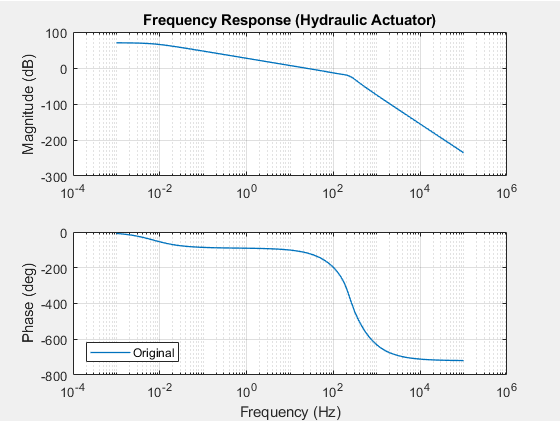
When the frequency, ω, is between 102 and 103 Hz, the phase drops by approximately 600 degrees. The rapid change in the phase shift, θ, indicates that the system has fast dynamics.
Calculate eigenvalues of the a matrix using the
eigfunction and plot the poles in the complex plane. Script for Calculating and Plotting the
A-Matrix Eigenvalues
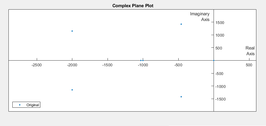
There are six fast poles, including two potential oscillating pole pairs.
Confirm that there are pole pairs. Print the values of the six fast poles to the command window using the
eigsfunction. Script for Printing Pole Values
ans =

   1.0e+03 *

  -2.0000 + 1.1547i
  -2.0000 - 1.1547i
  -0.4614 + 1.4208i
  -0.4614 - 1.4208i
  -1.0314 + 0.0000i
  -1.0000 + 0.0000i
There are two sets of pole pairs.
Identify and Eliminate the Sources of Fast Dynamics
Examine the model for potential sources of fast dynamics.
To linearize the model, this example uses the
linmodfunction. The documentation for thelinmodadvises against using the function to linearize a model that contains a Transport Delay block. The documentation for the Transport Delay block indicates that the Pade approximation for a linearization routine can add dynamic states to a model. Determine if the block is the source of the fast poles that result in the linearized model.To simulate the model without the effects of the Transport Delay block, comment through the block.
 Script for Commenting Out Transport Delay
Block
The icon for the Transport Delay fades to indicate that it is commented through.
To examine the frequency response of the model without the effects of the Transport Delay block, trim, linearize, and simulate the model, and then, update the Bode plot.
 Script for Trimming and Linearizing the Model and Updating the
Bode Plot
When the frequency, ω, is between 102 and 103 Hz, the phase drops by only by ~250 degrees.
Calculate and plot the fast poles.
 Script for Calculating and Plotting the
A-Matrix Eigenvalues
The Transport Delay block is responsible for the missing oscillatory pole pair at -2000 ± 1.1547i rad/sec
Plot the simulation results to see if they adequately match the original results.
 Script for Simulating the Model and Plotting the Results
The results appear similar.
Zoom to evaluate accuracy in more detail.
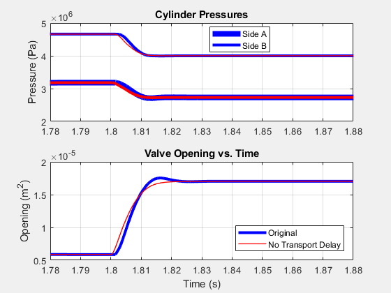
At this level, you can see a small difference in the results for the modified model. However, the simulation is accurate enough that the results meet expectations based on empirical and theoretical data.
The model includes hydraulic compressibility, that is, oil column resonance. To confirm that the column resonance is responsible for the second oscillatory pole pair, turn off compressibility and repeat the frequency response and pole analyses.
 Script for Eliminating Compressibility and Performing the
Frequency Response and Pole Analysis
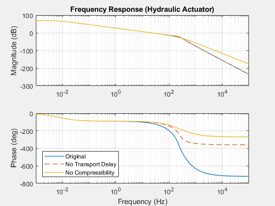

The further decrease in the phase drop reflects the reduction in high-frequency dynamics. There are now two fast poles. Even though one of the fast poles has moved further away from the imaginary axis, there are fewer fast dynamics because the oscillating pole pair at 458.8 ± 1.4273i rad/sec is eliminated.
Print the values of the remaining two fast poles to the command window.
 Script for Printing Pole Values
two_fast_poles =

   1.0e+03 *

   -2.6767
   -1.0000
The fast pole at -2677 rad/s corresponds to the load mass and hydraulic damping introduced by the two orifice components in the hydraulic subsystem. These dynamics are central to the simulation results. The fast pole at -1000 rad/s corresponds to the controller denominator, 0.001 s+1. The transfer function is integral to the controller design. No more dynamic modes can be removed without changing important system-level behavior.
Plot the simulation results to see if they adequately match the original results.
 Script for Plotting the Simulation Results
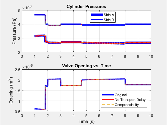
The accuracy of the updated model seems acceptable.
Zoom to evaluate accuracy in more detail.
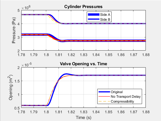
At this level, you can see that there is only a small additional difference in the results for the modified model. The accuracy of the simulation is acceptable.