为多输入多输出被控对象设计 ADRC

概述

在此示例中，被控对象是一个中试规模精馏塔模型 [1]。该模型有两个输入：磁通流量 ${\mathit{u}}_1$ 和蒸汽流量 ${\mathit{u}}_2$。该模型有两个输出：轻产物纯度 ${\mathit{y}}_1$ 和重产物纯度 ${\mathit{y}}_2$。该模型还包含未知扰动。

定义被控对象传递函数。

s = tf('s');
G = [12.8/(16.7*s+1),-18.9/(21*s+1);6.6/(10.9*s+1),-19.4/(14.4*s+1)];

控制器的目标是将输出保持为所需值 ${\mathit{r}}_1=0$ 和 ${\mathit{r}}_2=1$。要为被控对象设计两个 ADRC 控制器，您需要应用动态解耦控制方法 [1]。每个 ADRC 模块控制从输入 ${\mathit{u}}_{\mathit{i}}$ 到输出 ${\mathit{y}}_{\mathit{i}}$ ($\mathit{i}=1,2$) 的通道。然后，您设计一个模型预测控制器 (MPC) 作为 ADRC 设计性能的基准控制器。

设计 ADRC 控制器

要设计解耦的 ADRC 控制器，请按如下方式逼近双输入双输出被控对象模型。

其中：

要确定导数的阶数 ${\mathit{n}}_{\mathit{i}}$ 和临界增益 ${\mathit{b}}_{\mathit{i}}$，请在被控对象模型上执行阶跃输入试验。此示例提供了 DecoupledPlantIO 模型，用于对具有解耦输入和输出的模型进行仿真。

打开 Simulink® 模型。

mdl_step = "DecoupledPlantIO";
open_system(mdl_step)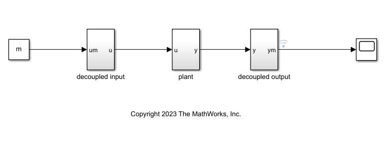

要执行从输入 ${\mathit{u}}_1=1$ 到输出 ${\mathit{y}}_1$ 的试验，请指定 m = 1。

对模型进行仿真并检查输出响应。

m = 1;
out = sim(mdl_step);
t1 = out.logsout{1}.Values.Time;
y1 = out.logsout{1}.Values.Data;
plot(t1,y1);
xlabel("time (s)")
ylabel("y1")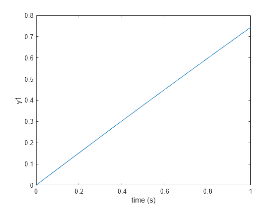

阶跃响应是一阶的，因此导数的阶数 ${\mathit{n}}_1=1$。您可以使用斜率来逼近临界增益 ${\mathit{b}}_1$。对于此响应，${\mathit{b}}_1=0.75$。

b1 = 0.75;

同样，为从输入 ${\mathit{u}}_2=1$ 到输出 ${\mathit{y}}_2$ 的试验指定 $\mathit{m}=2$。

m = 2;
out = sim(mdl_step);
t2 = out.logsout{1}.Values.Time;
y2 = out.logsout{1}.Values.Data;
plot(t2,y2);
xlabel('time (s)')
ylabel('y2')

阶跃响应也是一阶的，因此 ${\mathit{n}}_2=1$，临界增益 ${\mathit{b}}_2=-1.3$。

b2 = -1.3;

调节 ADRC 控制器

要调节 ADRC 控制器的性能，请使用控制器带宽 ${\mathit{w}}_{\mathit{c}}$ 和观测器带宽 ${\mathit{w}}_{\mathit{o}}$ 参数。在此示例中，调节目标是与最佳 MPC 控制器的性能匹配。

为被控对象模型设计 MPC 控制器。

Ts = 1; % sample time
mpc1 = mpc(G,Ts);

-->"PredictionHorizon" is empty. Assuming default 10.
-->"ControlHorizon" is empty. Assuming default 2.
-->"Weights.ManipulatedVariables" is empty. Assuming default 0.00000.
-->"Weights.ManipulatedVariablesRate" is empty. Assuming default 0.10000.
-->"Weights.OutputVariables" is empty. Assuming default 1.00000.

您可以调整控制器的权重以调节性能。有关详细信息，请参阅Tune Weights (Model Predictive Control Toolbox)。

指定 MPC 控制器的权重。

mpc1.Weights.ManipulatedVariablesRate = 0.7389*[1,1];
mpc1.Weights.OutputVariables = 0.1353*[1,1];

为了与 MPC 控制器的响应匹配，您必须设置 ADRC 控制器的控制器带宽和观测器带宽。对于此示例，${\mathit{w}}_{\mathit{c}}=0.25$ 和 ${\mathit{w}}_{\mathit{o}}=3$ 与 MPC 控制器的响应匹配。

wc = 0.25;
wo = 3;

运行模型 45 秒。

T = 45;
mdl = "ADRCWithBenchmarkMIMO";
open_system(mdl);

sim(mdl);

-->Converting the "Model.Plant" property to state-space.
-->Converting model to discrete time.
-->Assuming output disturbance added to measured output #1 is integrated white noise.
-->Assuming output disturbance added to measured output #2 is integrated white noise.

使用示波器查看被控对象的输出。

open_system(mdl + "/outputs")

MPC 控制器和 ADRC 控制器对输出 ${\mathit{y}}_2$ 的响应相似。与 MPC 控制器相比，ADRC 控制器对输出 ${\mathit{y}}_1$ 的跟踪误差更小。

抗扰

该模型具有 50 到 100 秒的外部扰动。将模型运行到 150 秒。

T = 150;
sim(mdl);

使用示波器查看被控对象的输出。

open_system(mdl + "/outputs")

对于此示例，与基准 MPC 控制器相比，ADRC 控制器具有更出色的抗扰结果。由于 ADRC 控制器使用幅值更大的控制输入，因此在存在扰动的情况下，输出会更快地收敛到参考值。使用示波器查看被控对象的输入。

open_system(mdl + "/inputs")

参考资料

[1] Zheng, Qing, Zhongzhou Chen, and Zhiqiang Gao.“A Dynamic Decoupling Control Approach and Its Applications to Chemical Processes.”In 2007 American Control Conference, 5176–81, 2007. https://doi.org/10.1109/ACC.2007.4282973.