Choose Mathematical Models that Represent Cables or Lines
This tutorial shows how to select a mathematical model for cables or lines for your application from different types of delay-based, lumped-parameter, and distributed models. First, the tutorial discusses the different models and compares the equations that they use. For a brief summary of the models, their intended applications, and the blocks that use them, see Summary of Mathematical Models.
To calculate the current through and voltage across cables and lines, you need to consider:
The distributed resistance of the conductors, R, which causes attenuation (signal loss), particularly at high currents and low frequencies.
The distributed inductance of the conductors, L, due to the magnetic field around the conductors and their self-inductance. Inductance slows down signal propagation because it resists changes in current. This effect is most pronounced for transient responses at high frequencies.
The distributed capacitance between pairs of conductors, C, which delays voltage changes when energy is stored in the electric field, especially at high frequencies and for shielded or coaxial cables.
The distributed conductance of the dielectric material separating pairs of conductors, G, which causes leakage and attenuation, especially at high voltage.
Choose a mathematical model based on the strength of each of these effects in your application and the arrangement of the conductors. In the simplest case, for short wires carrying a low current, you can treat R, L, C, and G as negligible. In this case, you can connect two blocks directly with physical connection lines to model a heavily idealized wire between them. In contrast, the most complex models treat R, L, C, and G as evenly distributed over the length of the conductors and dependent on the frequency of the signal. Simscape™ blocks use a range of simplifying assumptions between these two extremes. The resulting models, in order of increasing complexity, are delay-based models, lumped-parameter models, and distributed models.
Delay-Based Models
Delay-based models do not model inductance or capacitance explicitly, but instead represent their effects as a pure time delay. The simplest delay-based model ignores signal losses and treats the transmission line as a fixed impedance, irrespective of frequency, plus a delay term. The defining equations of the simplest delay-based model are
v1( t ) – i1( t ) Z0 = v2( t – τ ) + i2( t – τ ) Z0
v2( t ) – i2( t ) Z0 = v1( t – τ ) + i1( t – τ ) Z0,
where:
v1 is the voltage across the left-hand end of the transmission line.
i1 is the current into the left-hand end of the transmission line.
v2 is the voltage across the right-hand end of the transmission line.
i2 is the current into the right-hand end of the transmission line.
τ is the transmission line delay.
Z0 is the characteristic impedance of the transmission line.
To introduce losses, you can connect several delay-based components in series with resistors between them.
Delay-based models are useful for simplified timing analysis of high-speed digital
systems where the line delay dominates and there are no reflections or
frequency-dependent effects. To model a single-phase transmission line using a
delay-based model, use the Transmission Line block and set the Model Type
parameter to Delay-based and lossless or
Delay-based
                                                  and lossy
.
Lumped-Parameter Models
Lumped-parameter models simplify the cable or line by concentrating properties like resistance, inductance, and capacitance into a single point, instead of considering them as distributed along the length of the conductors. This enables you to model the cable or line as a simple equivalent circuit. Use this approach to create more manageable models, especially at lower frequencies where the effects of spatial distribution are less significant.
Most of the lumped-parameter models in Simscape divide the cable or line into series segments, each comprising resistors, inductors, and capacitors. The accuracy of these models increases with the number of segments and decreases with increases in line length or frequency. This approach is useful for modeling short- to medium-length cables or lines when detailed electromagnetic behavior is not required. For example, you can use this approach for capturing transient responses in DC systems, analyzing low-frequency AC systems, system-level modeling in power transmission and distribution applications, and fault analysis.
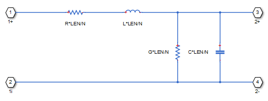
This figure shows the block diagram for an L-section segment. A series resistor with
resistance R*LEN/N, and inductor with inductance
L*LEN/N, model the inner conductor. A parallel resistor with
resistance G*LEN/N, and capacitor with capacitance
C*LEN/N, model the capacitance and leakage conductance, respectively,
between the inner conductor and the external shielding conductor. The physical
connection line between the Connection Port blocks
labeled +1 to 2+ represents the inner conductor.
The physical connection line between the Connection Port
blocks labeled 1i to 2- represents the external
shielding conductor.
Here:
R is line resistance per unit length.
L is the line inductance per unit length.
C is the line capacitance per unit length.
G is the line conductance per unit length.
LEN is the length of the line.
N is the number of series segments.
Lumped-parameter models vary in complexity depending on the number of conductors and the number and types of the passive elements incorporated into the equivalent circuit.
To model short conductors carrying low-frequency signals, a single segment with a resistor and an inductor is often sufficient. To model multiple conductors in a single cable, you can use the Cable and Connectors block. This block models each conductor as a series resistor and inductor. Optionally, it also models the connectors as resistors representing the contact resistance and inter-pin conductance.
To model a single-phase AC line with a central conductor and external shielding
conductor, you can use the Transmission Line block and set the Model Type
parameter to Lumped parameter L-section or
Lumped
                                                  parameter pi-section
. The pi-section model
incorporates an additional parallel inductor and capacitor into each L-section for
greater accuracy.
To model cables with more conducting layers or to model three-phase lines, you need additional passive elements in each section to account for the greater number of conductors.
The Transmission Line (Three-Phase) block models a three-phase transmission line using the lumped-parameter pi-line model. This model accounts for:
The resistance of each phase and the line-line mutual resistance
The self-inductance of each phase and the line-line mutual inductance
The line-line and line-ground capacitance
The Coupled Lines (Pair) and Coupled Lines (Three-Phase) blocks model magnetically-coupled instead of capacitively-coupled lines. These models are useful when magnetic coupling in the network is significant. These effects are most prominent when:
The lines are parallel and close together
The self-inductances of the lines are high
The AC frequency of the network is high
The AC Cable (Three-Phase) block models a three-phase power cable with central conductors and a conducting sheath surrounding each phase. The model accounts for:
The resistance of each phase and sheath and the return path.
The inductance of, and mutual inductance between, each phase, each sheath, and the return path.
The capacitance between each phase and the corresponding sheath.
The capacitance between each sheath and the return path.
You can also create your own lumped-parameter models using a combination of Resistor, Inductor, and Capacitor blocks or the RLC (Three-Phase) block. This approach is useful when you only need a simple model. For example:
A Resistor and Inductor block in series are sufficient to model a short conductor in DC or low-frequency applications.
Series segments of parallel Inductor and Capacitor blocks are sufficient to model short lines carrying high-frequency signals. For a simple model of a lossless transmission line, see LC Transmission Line and Test Bridge.
Creating custom models is also useful for modeling specialized cable arrangements and for modeling faults or thermal effects.
Distributed Models
Distributed models treat R, L, C, and G as being evenly distributed over the length of the conductors. These models then solve differential equations for voltage and current with respect to length along the conductors, x. This high-fidelity approach is useful for modeling long cables and lines, or for modeling short cables and lines when you need to capture detailed electromagnetic behavior. The telegrapher's equations describe the electromagnetic behavior of a multiconductor transmission line:
where:
V is the vector of line phase voltages.
I is the vector of phase currents.
Z is the series impedance matrix in per unit length.
Y is the shunt admittance matrix in per unit length.
For a single-phase line V, I, Z, and Y are scalars.
The Transmission Line block with the
Model Type parameter set to
Distributed parameter uses a distributed model to
represent a line with an inner conductor and external shielding conductor. This model is
not frequency-dependent. It is highly accurate, but only at a given frequency.
The DC Cable models a DC power cable with six concentric layers: core conductor, insulation, sheath, inner jacket, armor, and serving. The model uses a frequency-dependent approach. This block is useful for simulating transient responses with high precision in high-voltage direct-current (HVDC) transmission applications.
The Frequency-Dependent Overhead Line (Three-Phase) block models a three-phase line using a frequency-dependent distributed model. This block is useful for long-distance transmission lines with ground return, where behavior is highly frequency dependent.
Summary of Mathematical Models
This table summarizes the different types of models in increasing order of complexity. In this categorization, some models share the same level of fidelity but serve different purposes. Delay-based models focus on timing, whereas lumped-parameter models with series resistance and inductance focus on power. Similarly, lumped-parameter models with pi- or L-sections are effective at low frequencies, whereas lumped-parameter models that incorporate magnetic coupling, but do not model capacitance, are effective at high frequencies. Use this table to select a model for your application.
Fidelity Level | Model Type | Model Summary | Applications | Simscape Electrical Blocks |
| Very low | Ideal connection or lumped resistance |
|
|
|
| Low | Delay-based |
|
|
|
| Low | Lumped parameter with series RL only |
|
|
|
| Medium | Lumped parameter pi- or L-sections |
|
|
|
| Medium | Lumped-parameter with magnetically-coupled lines |
|
| |
| High | Distributed and frequency independent |
|
|
|
| Very high | Distributed and frequency dependent |
|
|
See Also
Simscape Blocks
- AC Cable (Three-Phase) | Cable and Connectors | Coupled Lines (Pair) | Coupled Lines (Three-Phase) | DC Cable | Frequency-Dependent Overhead Line (Three-Phase) | Transmission Line | Transmission Line (Three-Phase)