binningTabularSynthesizer
Description
To generate synthetic data, you can first create a
binningTabularSynthesizer object using an existing multivariate data set.
The object uses binning techniques to learn the distribution of the data set. Then, use the
synthesizeTabularData object function to synthesize data using the object. After
you synthesize data, you can test whether the new data set comes from the same distribution as
the original data set. Use the mmdtest or
knntest function to
determine how close the data distributions are to each other.
Creation
Syntax
Description
synthesizer = binningTabularSynthesizer(X)synthesizer) using the
existing data X.
synthesizer = binningTabularSynthesizer(___,Name=Value)
Input Arguments
Existing data set, specified as a numeric matrix or a table. Rows of
X correspond to observations, and columns of
X correspond to variables. Multicolumn variables and cell
arrays other than cell arrays of character vectors are not supported.
Data Types: single | double | table
Since R2026a
Name of the class labels variable in X, specified as a
character vector or string scalar. X must be a table, and
Yname must specify a column in X that is a
numeric, categorical, or logical vector; a character or string array; or a cell array
of character vectors. The Yname variable must contain class
labels for one or two classes only.
Data Types: char | string
Since R2026a
Class labels for one or two classes, specified as a numeric, categorical, or
logical vector; a character or string array; or a cell array of character vectors.
Rows of Y correspond to observations.
Data Types: single | double | logical | char | string | cell | categorical
Name-Value Arguments
Specify optional pairs of arguments as
Name1=Value1,...,NameN=ValueN, where Name is
the argument name and Value is the corresponding value.
Name-value arguments must appear after other arguments, but the order of the
pairs does not matter.
Example: binningTabularSynthesizer(X,BinMethod="equiprobable",NumBins=10)
specifies to use 10 equiprobable bins for each variable in
X.
Binning algorithm, specified as one of the values in this table. Note the following:
Xiis the existing data set for classiwhen you specify class labels for two classes. Otherwise, it is the existing data setX.miis the number of observations in the existing data for classiwhen you specify class labels for two classes. Otherwise, it is the number of observations in the existing data setX.
| Value | Description |
|---|---|
"auto" |
|
"equal-width" | Equal-width binning, where you must specify the number of bins
using the NumBins name-value argument |
"equiprobable" | Equiprobable binning, where you must specify the number of bins
using the NumBins name-value argument |
"dagostino-stephens" or
"ds" | Equiprobable binning with ceil(2*mi^(2/5))
bins |
"freedman-diaconis" or
"fd" | Equal-width binning, where each bin for variable
k has a width of
ceil(2*iqr(Xi(:,k))*mi^(-1/3)) |
"scott" | Equal-width binning, where each bin for variable
k has a width of
ceil(3.5*std(Xi(:,k))*mi^(-1/3)) |
"scott-multivariate" | Equal-width binning, where each bin for variable
k has a width of
3.5*std(Xi(:,k))*mi^(-1/(2+d)) |
"terrell-iqr" | Equal-width binning, where each bin for variable
k has a width of
2.603*iqr(Xi(:,k))*mi^(-1/3) |
"terrell-scott" or
"ts" | Equal-width binning with ceil((2*mi)^(1/3))
bins |
"terrell-std" | Equal-width binning, where each bin for variable
k has a width of
3.729*std(Xi(:,k))*mi^(-1/3) |
Example: BinMethod="scott"
Data Types: char | string
Number of bins to use for continuous variables, specified as a positive integer scalar or vector.
If
NumBinsis a scalar, then the function uses the same number of bins for each continuous variable.If
NumBinsis a vector, then the function usesNumBins(k)number of bins for continuous variablek.
Specify this value only when BinMethod is
"equal-width" or "equiprobable".
Example: NumBins=[10 25 10 15]
Data Types: single | double
Variable names, specified as a string array or a cell array of character vectors.
If
Xis a numeric matrix, then you can useVariableNamesto assign names to the variables inX.The order of the names in
VariableNamesmust correspond to the order of the variables inX. That is,VariableNames{1}is the name ofX(:,1),VariableNames{2}is the name ofX(:,2), and so on.size(X,2)andnumel(VariableNames)must be equal.By default,
VariableNamesis{'x1','x2',...}.
If
Xis a table, then you can useVariableNamesto choose which variables to use. That is,binningTabularSynthesizeruses only the variables inVariableNamesto generate synthetic data.VariableNamesmust be a subset ofX.Properties.VariableNames.By default,
VariableNamescontains the names of all variables, excluding the class labels variableYname.
Example: VariableNames=["SepalLength","SepalWidth","PetalLength","PetalWidth"]
Data Types: string | cell
List of the categorical variables, excluding the class labels variable
Yname, specified as one of the values in this table.
| Value | Description |
|---|---|
| Positive integer vector | Each entry in the vector is an index value indicating that the
corresponding variable is categorical. The index values are between 1 and
v, where v is the number of variables
listed in |
| Logical vector | A |
| String array or cell array of character vectors | Each element in the array is the name of a categorical variable. The names must
match the entries in VariableNames. |
"all" | All variables are categorical. |
By default, if the variables are in a numeric matrix, the software assumes all the variables
are continuous. If the variables are in a table, the software assumes they are
categorical if they are logical vectors, categorical vectors, character
arrays, string arrays, or cell arrays of character vectors. To identify any other
variables as categorical, specify them by using the
CategoricalVariables name-value argument.
Do not specify discrete numeric variables as categorical variables. Use the
DiscreteNumericVariables name-value argument instead.
Example: CategoricalVariables="all"
Data Types: single | double | logical | string | cell
List of the discrete numeric variables, specified as one of the values in this table.
| Value | Description |
|---|---|
| Positive integer vector | Each entry in the vector is an index value indicating that
the corresponding variable is a discrete numeric variable. The
index values are between 1 and v, where
v is the number of variables listed in
|
| Logical vector | A |
| String array or cell array of character vectors | Each element in the array is the name of a discrete numeric
variable. The names must match the entries in
VariableNames. |
"all" | All variables are discrete numeric variables. |
You cannot specify categorical variables as discrete numeric variables.
Example: DiscreteNumericVariables=[2 5]
Data Types: single | double | logical | string | cell
Properties
This property is read-only.
Variable names, returned as a string array. The order of the elements of
VariableNames corresponds to the order in which the variable
names appear in the existing data set X.
Data Types: string
This property is read-only.
Indices of the categorical variables, returned as a positive integer vector. Each
index value in CategoricalVariables indicates that the
corresponding variable listed in VariableNames
is categorical. If none of the variables are categorical, then this property is empty
([]).
Data Types: double
This property is read-only.
Indices of the discrete numeric variables, returned as a positive integer vector.
Each index value in DiscreteNumericVariables indicates that the
corresponding variable listed in VariableNames
is a discrete numeric variable. If none of the variables are discrete numeric variables,
then this property is empty ([]).
Data Types: double
This property is read-only.
Indices of the binned variables, returned as a positive integer vector. Each index
value in BinnedVariables indicates that the corresponding variable
listed in VariableNames
is a binned variable. If none of the variables are binned, then this property is empty
([]).
Data Types: double
This property is read-only.
Binning algorithm used to bin the continuous variables indicated by BinnedVariables, returned as "equal-width",
"equiprobable", "dagostino-stephens",
"freedman-diaconis", "scott",
"scott-multivariate", "terrell-iqr",
"terrell-scott", or "terrell-std". For more
information on these binning algorithms, see the BinMethod name-value argument.
If none of the variables are binned, then this property is empty.
Data Types: string
This property is read-only.
Number of bins used to bin the continuous variables, returned as a
1-by-k positive integer vector or a 2-by-k
positive integer matrix, where k is the number of variables in
BinnedVariables.
If
NumBinsis a vector, thenNumBins(j)indicates the number of bins for continuous variablej.If
NumBinsis a matrix, thenNumBins(i,j)indicates the number of bins for continuous variablejand classi. (since R2026a)
If none of the variables are binned, then this property is empty
([]).
Data Types: double
This property is read-only.
Bin edges used to bin the continuous variables, returned as a
1-by-k cell array or a 2-by-k cell array, where
k is the number of variables in BinnedVariables.
If
BinEdgesis a vector, thenBinEdges(j)contains the bin edges for continuous variablej.If
BinEdgesis a matrix, thenBinEdges(i,j)contains the bin edges for continuous variablejand classi. (since R2026a)
If none of the variables are binned, then this property is empty.
Data Types: cell
Since R2026a
This property is read-only.
Names of the classes in Yname or
Y for which
to generate synthetic data, returned as a numeric, categorical, or logical vector; a
character or string array; or a cell array of character vectors. If you do not specify
class labels when you create the synthesizer object, then this property is empty
([]).
Data Types: single | double | logical | char | string | cell | categorical
This property is read-only.
Number of observations in the existing data set X, returned
as a positive integer scalar or a two-element positive integer vector. If you specify
class labels when you create the synthesizer object, then
NumObservations(i) corresponds to the number of observations in the
existing data set that belong to class ClassNames(i,:).
Data Types: double
Object Functions
synthesizeTabularData | Synthesize tabular data using binning-based or SMOTE-based synthesizer |
Examples
Use existing training data to create a binningTabularSynthesizer object. Then, synthesize data using the synthesizeTabularData object function. Train a model using the existing training data, and then train the same type of model using the synthetic data. Compare the performance of the two models using test data.
Load the carbig data set, which contains measurements of cars made in the 1970s and early 1980s. Create a table containing the predictor variables Acceleration, Displacement, and so on, as well as the response variable MPG.
load carbig
tbl = table(Acceleration,Cylinders,Displacement,Horsepower, ...
    Model_Year,Origin,MPG,Weight);
Remove rows of tbl where the table has missing values.
tbl = rmmissing(tbl);
Partition the data into training and test sets. Use approximately 60% of the observations for model training and synthesizing new data, and 40% of the observations for model testing. Use cvpartition to partition the data.
rng("default")
cv = cvpartition(size(tbl,1),"Holdout",0.4);
trainTbl = tbl(training(cv),:);
testTbl = tbl(test(cv),:);
Create a binningTabularSynthesizer object by using the trainTbl data set. The binningTabularSynthesizer function uses binning techniques to learn the distribution of the multivariate data set. Use 20 equal-width bins for each continuous variable. Specify the Cylinders and Model_Year variables as discrete numeric variables.
synthesizer = binningTabularSynthesizer(trainTbl, ...
    BinMethod="equal-width",NumBins=20, ...
    DiscreteNumericVariables=["Cylinders","Model_Year"])
synthesizer =
  binningTabularSynthesizer

               VariableNames: ["Acceleration"    "Cylinders"    "Displacement"    "Horsepower"    "Model_Year"    "Origin"    "MPG"    "Weight"]
        CategoricalVariables: 6
    DiscreteNumericVariables: [2 5]
             BinnedVariables: [1 3 4 7 8]
                   BinMethod: "equal-width"
                     NumBins: [20 20 20 20 20]
                    BinEdges: {[21×1 double]  [21×1 double]  [21×1 double]  [21×1 double]  [21×1 double]}
             NumObservations: 236


  Properties, Methods
synthesizer is a binningTabularSynthesizer object with five binned variables. Each binned variable has the same number of bins.
Synthesize new data by using synthesizer. Specify to generate 1000 observations.
syntheticTbl = synthesizeTabularData(synthesizer,1000);
The synthesizeTabularData object function uses the data distribution information stored in synthesizer to generate syntheticTbl.
To visualize the difference between the existing data and synthetic data, you can use the detectdrift function. The function uses permutation testing to detect drift between trainTbl and syntheticTbl.
dd = detectdrift(trainTbl,syntheticTbl);
dd is a DriftDiagnostics object with plotEmpiricalCDF and plotHistogram object functions for visualization.
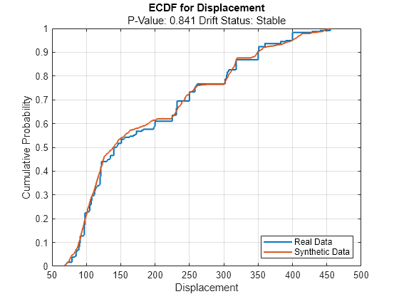
For continuous variables, use the plotEmpiricalCDF function to see the difference between the empirical cumulative distribution function (ecdf) of the values in trainTbl and the ecdf of the values in syntheticTbl.
continuousVariable ="Displacement"; plotEmpiricalCDF(dd,Variable=continuousVariable) legend(["Real data","Synthetic data"])

For the Displacement predictor, the ecdf plot for the existing values (in blue) matches the ecdf plot for the synthetic values (in red) fairly well.
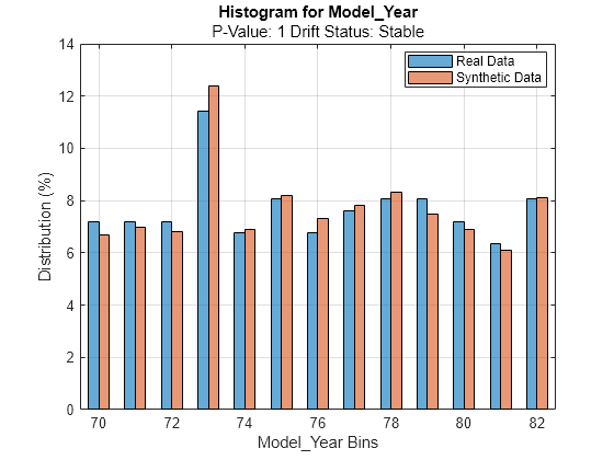
For discrete variables, use the plotHistogram function to see the difference between the histogram of the values in trainTbl and the histogram of the values in syntheticTbl.
discreteVariable ="Model_Year"; plotHistogram(dd,Variable=discreteVariable) legend(["Real data","Synthetic data"])

For the Model_Year predictor, the histogram for the existing values (in blue) matches the histogram for the synthetic values (in red) fairly well.
Train a bagged ensemble of trees using the original training data trainTbl. Specify MPG as the response variable. Then, train the same kind of regression model using the synthetic data syntheticTbl.
originalMdl = fitrensemble(trainTbl,"MPG",Method="Bag");
newMdl = fitrensemble(syntheticTbl,"MPG",Method="Bag");
Evaluate the performance of the two models on the test set by computing the test mean squared error (MSE). Smaller MSE values indicate better performance.
originalMSE = loss(originalMdl,testTbl)
originalMSE =
7.0784
newMSE = loss(newMdl,testTbl)
newMSE =
6.1031
The model trained on the synthetic data performs slightly better on the test data.
Evaluate data synthesized from an existing data set. Compare the existing and synthetic data sets to determine the similarity between the two multivariate data distributions.
Load the sample file fisheriris.csv, which contains iris data including sepal length, sepal width, petal width, and species type. Read the file into a table, and then convert the Species variable into a categorical variable. Print a summary of the variables in the table.
fisheriris = readtable("fisheriris.csv");
fisheriris.Species = categorical(fisheriris.Species);
summary(fisheriris)
fisheriris: 150×5 table
Variables:
SepalLength: double
SepalWidth: double
PetalLength: double
PetalWidth: double
Species: categorical (3 categories)
Statistics for applicable variables:
NumMissing Min Median Max Mean Std
SepalLength 0 4.3000 5.8000 7.9000 5.8433 0.8281
SepalWidth 0 2 3 4.4000 3.0573 0.4359
PetalLength 0 1 4.3500 6.9000 3.7580 1.7653
PetalWidth 0 0.1000 1.3000 2.5000 1.1993 0.7622
Species 0
The summary display includes statistics for each variable. For example, the sepal length values range from 4.3 to 7.9, with a median of 5.8.
Create 150 new observations from the data in fisheriris. First, create an object by using the binningTabularSynthesizer function. Then, synthesize the data by using the synthesizeTabularData object function. Print a summary of the variables in the new syntheticData data set.
rng(0,"twister") % For reproducibility
synthesizer = binningTabularSynthesizer(fisheriris);
syntheticData = synthesizeTabularData(synthesizer,150);
summary(syntheticData)
syntheticData: 150×5 table

Variables:

    SepalLength: double
    SepalWidth: double
    PetalLength: double
    PetalWidth: double
    Species: categorical (3 categories)

Statistics for applicable variables:

                   NumMissing       Min          Median         Max           Mean          Std

    SepalLength        0           4.3079        5.7174        7.6399        5.8280        0.8576
    SepalWidth         0           2.0236        3.0336        4.2866        3.0819        0.4572
    PetalLength        0           1.0010        4.4453        6.8538        3.6572        1.8192
    PetalWidth         0           0.1002        1.3502        2.4759        1.1719        0.7597
    Species            0
You can compare the variable statistics for syntheticData to the variable statistics for fisheriris. For example, the sepal length values in the synthetic data set range from approximately 4.3 to 7.6, with a median of 5.7. These statistics are similar to the statistics in the fisheriris data set.
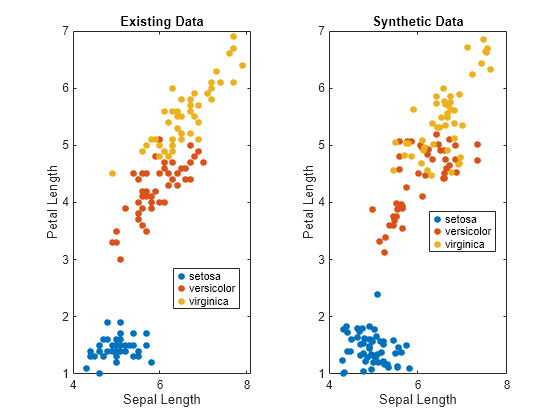
Visually compare the observations in fisheriris and syntheticData by using scatter plots. Each point corresponds to an observation. The point color indicates the species of the corresponding iris.
tiledlayout(1,2)
nexttile
gscatter(fisheriris.SepalLength,fisheriris.PetalLength,fisheriris.Species)
xlabel("Sepal Length")
ylabel("Petal Length")
title("Existing Data")
nexttile
gscatter(syntheticData.SepalLength,syntheticData.PetalLength,syntheticData.Species)
xlabel("Sepal Length")
ylabel("Petal Length")
title("Synthetic Data")

The scatter plots indicate that the existing data set and the synthetic data set have similar characteristics.
Compare the existing and synthetic data sets by using the mmdtest function. The function performs a two-sample hypothesis test for the null hypothesis that the data sets come from the same distribution.
[mmd2,p,h] = mmdtest(fisheriris,syntheticData)
mmd2 =
0.0020
p =
0.9600
h =
0
The returned value of h = 0 indicates that mmdtest fails to reject the null hypothesis that the data sets come from different distributions at the significance level of 5%. As with other hypothesis tests, this result does not guarantee that the null hypothesis is true. That is, the data sets do not necessarily come from the same distribution, but the low mmd2 value (square maximum mean discrepancy) and the high p-value indicate that the distributions of the real and synthetic data sets are similar.
Algorithms
When you use a binning technique, the binningTabularSynthesizer function estimates the
distribution of the multivariate data set X by performing these steps:
Bin each continuous variable using equiprobable or equal-width binning, as specified by the
BinMethodandNumBinsname-value arguments.Encode the continuous variables using the bin indices.
One-hot encode all binned and discrete variables.
Compute the probability of each unique row in the encoded data set.
If you specify class labels for two classes (using
Yname or Y), the function estimates the
distribution for each data set X1 and X2, where X1 contains the observations in the first class and X2 contains the observations in the second class. (since R2026a)
The synthesizeTabularData function uses the computed probabilities to
generate synthetic data.
Alternative Functionality
Instead of creating a binningTabularSynthesizer object and then using the
synthesizeTabularData object function to synthesize data, you can generate
synthetic data directly by using the synthesizeTabularData function. Create an object if you want to easily generate
synthetic data multiple times without having to relearn characteristics of the existing data
set.
Version History
Introduced in R2024bWhen you use a binningTabularSynthesizer object, the synthesizeTabularData object function can return synthetic observations for
one or two classes. Use the Yname or Y input
argument when you create the object, and the ClassNames name-value
argument when you call synthesizeTabularData.
See Also
synthesizeTabularData | mmdtest | knntest | detectdrift | plotEmpiricalCDF | plotHistogram | synthesizeTabularData
MATLAB Command
You clicked a link that corresponds to this MATLAB command:
Run the command by entering it in the MATLAB Command Window. Web browsers do not support MATLAB commands.
选择网站
选择网站以获取翻译的可用内容,以及查看当地活动和优惠。根据您的位置,我们建议您选择:。
您也可以从以下列表中选择网站:
如何获得最佳网站性能
选择中国网站(中文或英文)以获得最佳网站性能。其他 MathWorks 国家/地区网站并未针对您所在位置的访问进行优化。
美洲
- América Latina (Español)
- Canada (English)
- United States (English)
欧洲
- Belgium (English)
- Denmark (English)
- Deutschland (Deutsch)
- España (Español)
- Finland (English)
- France (Français)
- Ireland (English)
- Italia (Italiano)
- Luxembourg (English)
- Netherlands (English)
- Norway (English)
- Österreich (Deutsch)
- Portugal (English)
- Sweden (English)
- Switzerland
- United Kingdom (English)