kfoldMargin

Classification margins for cross-validated ECOC model

Syntax

margin = kfoldMargin(CVMdl)

margin = kfoldMargin(CVMdl,Name,Value)

Description

margin = kfoldMargin(CVMdl) returns classification margins obtained by the cross-validated ECOC model (ClassificationPartitionedECOC) CVMdl. For every fold, kfoldMargin computes classification margins for validation-fold observations using an ECOC model trained on training-fold observations. CVMdl.X contains both sets of observations.

example

margin = kfoldMargin(CVMdl,Name,Value) returns classification margins with additional options specified by one or more name-value pair arguments. For example, specify the binary learner loss function, decoding scheme, or verbosity level.

example

Examples

collapse all

Estimate k-Fold Cross-Validation Margins

Open Live Script

Load Fisher's iris data set. Specify the predictor data X, the response data Y, and the order of the classes in Y.

load fisheriris
X = meas;
Y = categorical(species);
classOrder = unique(Y);
rng(1); % For reproducibility

Train and cross-validate an ECOC model using support vector machine (SVM) binary classifiers. Standardize the predictor data using an SVM template, and specify the class order.

t = templateSVM('Standardize',1);
CVMdl = fitcecoc(X,Y,'CrossVal','on','Learners',t,'ClassNames',classOrder);

CVMdl is a ClassificationPartitionedECOC model. By default, the software implements 10-fold cross-validation. You can specify a different number of folds using the 'KFold' name-value pair argument.

Estimate the margins for validation-fold observations. Display the distribution of the margins using a box plot.

margin = kfoldMargin(CVMdl);

boxplot(margin)
title('Distribution of Margins')

Figure contains an axes object. The axes object with title Distribution of Margins contains 7 objects of type line. One or more of the lines displays its values using only markers

Select ECOC Model Features by Comparing Cross-Validation Margins

Open Live Script

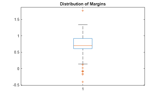
One way to perform feature selection is to compare cross-validation margins from multiple models. Based solely on this criterion, the classifier with the greatest margins is the best classifier.

Load Fisher's iris data set. Specify the predictor data X, the response data Y, and the order of the classes in Y.

load fisheriris
X = meas;
Y = categorical(species);
classOrder = unique(Y); % Class order
rng(1); % For reproducibility

Define the following two data sets.

fullX contains all the predictors.
partX contains the petal dimensions.

fullX = X;
partX = X(:,3:4);

For each predictor set, train and cross-validate an ECOC model using SVM binary classifiers. Standardize the predictors using an SVM template, and specify the class order.

t = templateSVM('Standardize',1);
CVMdl = fitcecoc(fullX,Y,'CrossVal','on','Learners',t,...
    'ClassNames',classOrder);
PCVMdl = fitcecoc(partX,Y,'CrossVal','on','Learners',t,...
    'ClassNames',classOrder);

CVMdl and PCVMdl are ClassificationPartitionedECOC models. By default, the software implements 10-fold cross-validation.

Estimate the margins for each classifier. Use loss-based decoding for aggregating the binary learner results. For each model, display the distribution of the margins using a boxplot.

fullMargins = kfoldMargin(CVMdl,'Decoding','lossbased');
partMargins = kfoldMargin(PCVMdl,'Decoding','lossbased');

boxplot([fullMargins partMargins],'Labels',{'All Predictors','Two Predictors'})
title('Distributions of Margins')

Figure contains an axes object. The axes object with title Distributions of Margins contains 14 objects of type line. One or more of the lines displays its values using only markers

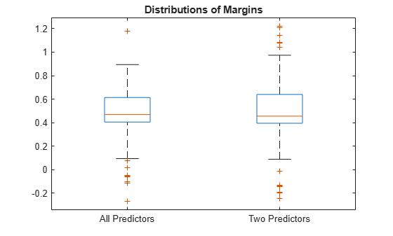
The margin distributions are approximately the same.

Input Arguments

collapse all

`CVMdl` — Cross-validated ECOC model
`ClassificationPartitionedECOC` model

Cross-validated ECOC model, specified as a ClassificationPartitionedECOC model. You can create a ClassificationPartitionedECOC model in two ways:

Pass a trained ECOC model (ClassificationECOC) to crossval.
Train an ECOC model using fitcecoc and specify any one of these cross-validation name-value pair arguments: 'CrossVal', 'CVPartition', 'Holdout', 'KFold', or 'Leaveout'.

Name-Value Arguments

collapse all

Specify optional pairs of arguments as Name1=Value1,...,NameN=ValueN, where Name is the argument name and Value is the corresponding value. Name-value arguments must appear after other arguments, but the order of the pairs does not matter.

Before R2021a, use commas to separate each name and value, and enclose Name in quotes.

Example: kfoldMargin(CVMdl,'Verbose',1) specifies to display diagnostic messages in the Command Window.

`BinaryLoss` — Binary learner loss function
`'hamming'` | `'linear'` | `'logit'` | `'exponential'` | `'binodeviance'` | `'hinge'` | `'quadratic'` | function handle

Binary learner loss function, specified as the comma-separated pair consisting of 'BinaryLoss' and a built-in loss function name or function handle.

This table describes the built-in functions, where y_j is the class label for a particular binary learner (in the set {–1,1,0}), s_j is the score for observation j, and g(y_j,s_j) is the binary loss formula.

Value	Description	Score Domain	g(y_j,s_j)
`"binodeviance"`	Binomial deviance	(–∞,∞)	log[1 + exp(–2y_js_j)]/[2log(2)]
`"exponential"`	Exponential	(–∞,∞)	exp(–y_js_j)/2
`"hamming"`	Hamming	[0,1] or (–∞,∞)	[1 – sign(y_js_j)]/2
`"hinge"`	Hinge	(–∞,∞)	max(0,1 – y_js_j)/2
`"linear"`	Linear	(–∞,∞)	(1 – y_js_j)/2
`"logit"`	Logistic	(–∞,∞)	log[1 + exp(–y_js_j)]/[2log(2)]
`"quadratic"`	Quadratic	[0,1]	[1 – y_j(2s_j – 1)]²/2

The software normalizes binary losses so that the loss is 0.5 when y_j = 0. Also, the software calculates the mean binary loss for each class [1].

For a custom binary loss function, for example customFunction, specify its function handle 'BinaryLoss',@customFunction.
customFunction has this form:
```
bLoss = customFunction(M,s)
```
- M is the K-by-B coding matrix stored in Mdl.CodingMatrix.
- s is the 1-by-B row vector of classification scores.
- bLoss is the classification loss. This scalar aggregates the binary losses for every learner in a particular class. For example, you can use the mean binary loss to aggregate the loss over the learners for each class.
- K is the number of classes.
- B is the number of binary learners.
For an example of passing a custom binary loss function, see Predict Test-Sample Labels of ECOC Model Using Custom Binary Loss Function.

This table identifies the default BinaryLoss value, which depends on the score ranges returned by the binary learners.

Assumption	Default Value
All binary learners are any of the following: Classification decision trees Discriminant analysis models k-nearest neighbor models Naive Bayes models	`'quadratic'`
All binary learners are SVMs.	`'hinge'`
All binary learners are ensembles trained by `AdaboostM1` or `GentleBoost`.	`'exponential'`
All binary learners are ensembles trained by `LogitBoost`.	`'binodeviance'`
You specify to predict class posterior probabilities by setting `'FitPosterior',true` in `fitcecoc`.	`'quadratic'`
Binary learners are heterogeneous and use different loss functions.	`'hamming'`

To check the default value, use dot notation to display the BinaryLoss property of the trained model at the command line.

Example: 'BinaryLoss','binodeviance'

Data Types: char | string | function_handle

`Decoding` — Decoding scheme
`'lossweighted'` (default) | `'lossbased'`

Decoding scheme that aggregates the binary losses, specified as the comma-separated pair consisting of 'Decoding' and 'lossweighted' or 'lossbased'. For more information, see Binary Loss.

Example: 'Decoding','lossbased'

`Options` — Estimation options
`[]` (default) | structure array

Estimation options, specified as a structure array as returned by statset.

To invoke parallel computing you need a Parallel Computing Toolbox™ license.

Example: Options=statset(UseParallel=true)

Data Types: struct

`Verbose` — Verbosity level
`0` (default) | `1`

Verbosity level, specified as 0 or 1. Verbose controls the number of diagnostic messages that the software displays in the Command Window.

If Verbose is 0, then the software does not display diagnostic messages. Otherwise, the software displays diagnostic messages.

Example: Verbose=1

Data Types: single | double

Output Arguments

collapse all

`margin` — Classification margins
numeric vector

Classification margins, returned as a numeric vector. margin is an n-by-1 vector, where each row is the margin of the corresponding observation and n is the number of observations (size(CVMdl.X,1)).

More About

collapse all

Classification Margin

The classification margin is, for each observation, the difference between the negative loss for the true class and the maximal negative loss among the false classes. If the margins are on the same scale, then they serve as a classification confidence measure. Among multiple classifiers, those that yield greater margins are better.

Binary Loss

The binary loss is a function of the class and classification score that determines how well a binary learner classifies an observation into the class. The decoding scheme of an ECOC model specifies how the software aggregates the binary losses and determines the predicted class for each observation.

Assume the following:

m_kj is element (k,j) of the coding design matrix M—that is, the code corresponding to class k of binary learner j. M is a K-by-B matrix, where K is the number of classes, and B is the number of binary learners.
s_j is the score of binary learner j for an observation.
g is the binary loss function.
$\hat{k}$ is the predicted class for the observation.

The software supports two decoding schemes:

Loss-based decoding [2] (Decoding is "lossbased") — The predicted class of an observation corresponds to the class that produces the minimum average of the binary losses over all binary learners.

$\hat{k} = \underset{k}{argmin} \frac{1}{B} \sum_{j = 1}^{B} | m_{k j} | g (m_{k j}, s_{j}) .$
Loss-weighted decoding [3] (Decoding is "lossweighted") — The predicted class of an observation corresponds to the class that produces the minimum average of the binary losses over the binary learners for the corresponding class.

$\hat{k} = \underset{k}{argmin} \frac{\sum_{j = 1}^{B} | m_{k j} | g (m_{k j}, s_{j})}{\sum_{j = 1}^{B} | m_{k j} |} .$
The denominator corresponds to the number of binary learners for class k. [1] suggests that loss-weighted decoding improves classification accuracy by keeping loss values for all classes in the same dynamic range.

The predict, resubPredict, and kfoldPredict functions return the negated value of the objective function of argmin as the second output argument (NegLoss) for each observation and class.

This table summarizes the supported binary loss functions, where y_j is a class label for a particular binary learner (in the set {–1,1,0}), s_j is the score for observation j, and g(y_j,s_j) is the binary loss function.

Value	Description	Score Domain	g(y_j,s_j)
`"binodeviance"`	Binomial deviance	(–∞,∞)	log[1 + exp(–2y_js_j)]/[2log(2)]
`"exponential"`	Exponential	(–∞,∞)	exp(–y_js_j)/2
`"hamming"`	Hamming	[0,1] or (–∞,∞)	[1 – sign(y_js_j)]/2
`"hinge"`	Hinge	(–∞,∞)	max(0,1 – y_js_j)/2
`"linear"`	Linear	(–∞,∞)	(1 – y_js_j)/2
`"logit"`	Logistic	(–∞,∞)	log[1 + exp(–y_js_j)]/[2log(2)]
`"quadratic"`	Quadratic	[0,1]	[1 – y_j(2s_j – 1)]²/2

The software normalizes binary losses so that the loss is 0.5 when y_j = 0, and aggregates using the average of the binary learners [1].

Do not confuse the binary loss with the overall classification loss (specified by the LossFun name-value argument of the kfoldLoss and kfoldPredict object functions), which measures how well an ECOC classifier performs as a whole.

References

[1] Allwein, E., R. Schapire, and Y. Singer. “Reducing multiclass to binary: A unifying approach for margin classiﬁers.” Journal of Machine Learning Research. Vol. 1, 2000, pp. 113–141.

[2] Escalera, S., O. Pujol, and P. Radeva. “Separability of ternary codes for sparse designs of error-correcting output codes.” Pattern Recog. Lett. Vol. 30, Issue 3, 2009, pp. 285–297.

[3] Escalera, S., O. Pujol, and P. Radeva. “On the decoding process in ternary error-correcting output codes.” IEEE Transactions on Pattern Analysis and Machine Intelligence. Vol. 32, Issue 7, 2010, pp. 120–134.

Extended Capabilities

expand all

Automatic Parallel Support
Accelerate code by automatically running computation in parallel using Parallel Computing Toolbox™.

To run in parallel, specify the Options name-value argument in the call to this function and set the UseParallel field of the options structure to true using statset:

Options=statset(UseParallel=true)

For more information about parallel computing, see Run MATLAB Functions with Automatic Parallel Support (Parallel Computing Toolbox).

GPU Arrays
Accelerate code by running on a graphics processing unit (GPU) using Parallel Computing Toolbox™.

This function fully supports GPU arrays. For more information, see Run MATLAB Functions on a GPU (Parallel Computing Toolbox).

Version History

Introduced in R2014b

kfoldMargin

Syntax

Description

Examples

Estimate k-Fold Cross-Validation Margins

Select ECOC Model Features by Comparing Cross-Validation Margins

Input Arguments

CVMdl — Cross-validated ECOC model ClassificationPartitionedECOC model

Name-Value Arguments

BinaryLoss — Binary learner loss function 'hamming' | 'linear' | 'logit' | 'exponential' | 'binodeviance' | 'hinge' | 'quadratic' | function handle

Decoding — Decoding scheme 'lossweighted' (default) | 'lossbased'

Options — Estimation options [] (default) | structure array

Verbose — Verbosity level 0 (default) | 1

Output Arguments

margin — Classification margins numeric vector

More About

Classification Margin

Binary Loss

References

Extended Capabilities

Automatic Parallel Support Accelerate code by automatically running computation in parallel using Parallel Computing Toolbox™.

GPU Arrays Accelerate code by running on a graphics processing unit (GPU) using Parallel Computing Toolbox™.

Version History

See Also

`CVMdl` — Cross-validated ECOC model
`ClassificationPartitionedECOC` model

`BinaryLoss` — Binary learner loss function
`'hamming'` | `'linear'` | `'logit'` | `'exponential'` | `'binodeviance'` | `'hinge'` | `'quadratic'` | function handle

`Decoding` — Decoding scheme
`'lossweighted'` (default) | `'lossbased'`

`Options` — Estimation options
`[]` (default) | structure array

`Verbose` — Verbosity level
`0` (default) | `1`

`margin` — Classification margins
numeric vector

Automatic Parallel Support
Accelerate code by automatically running computation in parallel using Parallel Computing Toolbox™.

GPU Arrays
Accelerate code by running on a graphics processing unit (GPU) using Parallel Computing Toolbox™.