Main Content

lillietest

Lilliefors test

Description

h = lillietest(x) returns a test decision for the null hypothesis that the data in vector x comes from a distribution in the normal family, against the alternative that it does not come from such a distribution, using a Lilliefors test. The result h is 1 if the test rejects the null hypothesis at the 5% significance level, and 0 otherwise.

example

h = lillietest(x,Name,Value) returns a test decision with additional options specified by one or more name-value pair arguments. For example, you can test the data against a different distribution family, change the significance level, or calculate the p-value using a Monte Carlo approximation.

example

[h,p] = lillietest(___) also returns the p-value p, using any of the input arguments from the previous syntaxes.

example

[h,p,kstat,critval] = lillietest(___) also returns the test statistic kstat and the critical value critval for the test.

example

Examples

collapse all

Load the sample data. Test the null hypothesis that car mileage, in miles per gallon (MPG), follows a normal distribution across different makes of cars.

load carbig
[h,p,k,c] = lillietest(MPG)
Warning: P is less than the smallest tabulated value, returning 0.001.
h = 
1
p = 
1.0000e-03
k = 
0.0789
c = 
0.0451

The test statistic k is greater than the critical value c, so lillietest returns a result of h = 1 to indicate rejection of the null hypothesis at the default 5% significance level. The warning indicates that the returned p-value is less than the smallest value in the table of precomputed values. To find a more accurate p-value, use MCTol to run a Monte Carlo approximation. See Determine the p-value Using Monte Carlo Approximation.

Load the sample data. Create a vector containing the first column of the students’ exam grades data.

load examgrades
x = grades(:,1);

Test the null hypothesis that the sample data comes from a normal distribution at the 1% significance level.

[h,p] = lillietest(x,'Alpha',0.01)
h = 
0
p = 
0.0348

The returned value of h = 0 indicates that lillietest does not reject the null hypothesis at the 1% significance level.

Load the sample data. Test the null hypothesis that car mileage, in miles per gallon (MPG), follows an exponential distribution across different makes of cars.

load carbig
h = lillietest(MPG,'Distribution','exponential')
h = 
1

The returned value of h = 1 indicates that lillietest rejects the null hypothesis at the default 5% significance level.

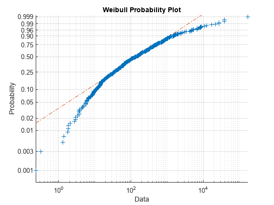
Generate two sample data sets, one from a Weibull distribution and another from a lognormal distribution. Perform the Lilliefors test to assess whether each data set is from a Weibull distribution. Confirm the test decision by performing a visual comparison using a Weibull probability plot (wblplot).

Generate samples from a Weibull distribution.

rng('default')
data1 = wblrnd(0.5,2,[500,1]);

Perform the Lilliefors test by using the lillietest. To test data for a Weibull distribution, test if the logarithm of the data has an extreme value distribution.

h1 = lillietest(log(data1),'Distribution','extreme value')
h1 = 
0

The returned value of h1 = 0 indicates that lillietest fails to reject the null hypothesis at the default 5% significance level. Confirm the test decision using a Weibull probability plot.

wblplot(data1)

Figure contains an axes object. The axes object with title Weibull Probability Plot, xlabel Data, ylabel Probability contains 3 objects of type line. One or more of the lines displays its values using only markers

The plot indicates that the data follows a Weibull distribution.

Generate samples from a lognormal distribution.

data2 =lognrnd(5,2,[500,1]);

Perform the Lilliefors test.

h2 = lillietest(log(data2),'Distribution','extreme value')
h2 = 
1

The returned value of h2 = 1 indicates that lillietest rejects the null hypothesis at the default 5% significance level. Confirm the test decision using a Weibull probability plot.

wblplot(data2)

Figure contains an axes object. The axes object with title Weibull Probability Plot, xlabel Data, ylabel Probability contains 3 objects of type line. One or more of the lines displays its values using only markers

The plot indicates that the data does not follow a Weibull distribution.

Load the sample data. Test the null hypothesis that car mileage, in miles per gallon (MPG), follows a normal distribution across different makes of cars. Determine the p-value using a Monte Carlo approximation with a maximum Monte Carlo standard error of 1e-4.

load carbig
[h,p] = lillietest(MPG,'MCTol',1e-4)
h = 
1
p = 
8.3333e-06

The returned value of h = 1 indicates that lillietest rejects the null hypothesis that the data comes from a normal distribution at the 5% significance level.

Input Arguments

collapse all

Sample data, specified as a vector.

Data Types: single | double

Name-Value Arguments

Specify optional pairs of arguments as Name1=Value1,...,NameN=ValueN, where Name is the argument name and Value is the corresponding value. Name-value arguments must appear after other arguments, but the order of the pairs does not matter.

Before R2021a, use commas to separate each name and value, and enclose Name in quotes.

Example: 'Distribution','exponential','Alpha',0.01 tests the null hypothesis that the population distribution belongs to the exponential distribution family at the 1% significance level.

Significance level of the hypothesis test, specified as the comma-separated pair consisting of 'Alpha' and a scalar value in the range (0,1).

  • If MCTol is not used, Alpha must be in the range [0.001,0.50].

  • If MCTol is used, Alpha must be in the range (0,1).

Example: 'Alpha',0.01

Data Types: single | double

Distribution family for the hypothesis test, specified as the comma-separated pair consisting of 'Distr' and one of the following.

'normal'Normal distribution
'exponential'Exponential distribution
'extreme value'Extreme value distribution

  • To test x for a lognormal distribution, test if log(x) has a normal distribution.

  • To test x for a Weibull distribution, test if log(x) has an extreme value distribution.

Example: 'Distribution','exponential'

Maximum Monte Carlo standard error for p, the p-value of the test, specified as the comma-separated pair consisting of 'MCTol' and a scalar value in the range (0,1).

Example: 'MCTol',0.001

Data Types: single | double

Output Arguments

collapse all

Hypothesis test result, returned as 1 or 0.

  • A value of 1 indicates the rejection of the null hypothesis at the Alpha significance level.

  • A value of 0 indicates a failure to reject the null hypothesis at the Alpha significance level.

p-value of the test, returned as a scalar value in the range (0,1). p is the probability of observing a test statistic as extreme as, or more extreme than, the observed value under the null hypothesis. Small values of p cast doubt on the validity of the null hypothesis.

  • If MCTol is not used, p is computed using inverse interpolation into the table of critical values, and is returned as a scalar value in the range [0.001,0.50]. lillietest warns when p is not found within the tabulated range and returns either the smallest or largest tabulated value.

  • If MCTol is used, lillietest conducts a Monte Carlo simulation to compute a more accurate p-value, and p is returned as a scalar value in the range (0,1).

Test statistic, returned as a nonnegative scalar value.

Critical value for the hypothesis test, returned as a nonnegative scalar value.

More About

collapse all

Lilliefors Test

The Lilliefors test is a two-sided goodness-of-fit test suitable when the parameters of the null distribution are unknown and must be estimated. This is in contrast to the one-sample Kolmogorov-Smirnov test, which requires the null distribution to be completely specified.

The Lilliefors test statistic is:

D*=maxx|F^(x)G(x)|,

where F^(x) is the empirical cdf of the sample data and G(x) is the cdf of the hypothesized distribution with estimated parameters equal to the sample parameters.

lillietest can be used to test whether the data vector x has a lognormal or Weibull distribution by applying a transformation to the data vector and running the appropriate Lilliefors test:

  • To test x for a lognormal distribution, test if log(x) has a normal distribution.

  • To test x for a Weibull distribution, test if log(x) has an extreme value distribution.

The Lilliefors test cannot be used when the null hypothesis is not a location-scale family of distributions.

Monte Carlo Standard Error

The Monte Carlo standard error is the error due to simulating the p-value.

The Monte Carlo standard error is calculated as:

SE=(p^)(1p^)mcreps,

where p^ is the estimated p-value of the hypothesis test, and mcreps is the number of Monte Carlo replications performed.

The number of Monte Carlo replications, mcreps, is determined such that the Monte Carlo standard error for p^ less than the value specified for MCTol.

Algorithms

To compute the critical value for the hypothesis test, lillietest interpolates into a table of critical values pre-computed using Monte Carlo simulation for sample sizes less than 1000 and significance levels between 0.001 and 0.50. The table used by lillietest is larger and more accurate than the table originally introduced by Lilliefors. If a more accurate p-value is desired, or if the desired significance level is less than 0.001 or greater than 0.50, the MCTol input argument can be used to run a Monte Carlo simulation to calculate the p-value more exactly.

When the computed value of the test statistic is greater than the critical value, lillietest rejects the null hypothesis at significance level Alpha.

lillietest treats NaN values in x as missing values and ignores them.

References

[1] Conover, W. J. Practical Nonparametric Statistics. Hoboken, NJ: John Wiley & Sons, Inc., 1980.

[2] Lilliefors, H. W. “On the Kolmogorov-Smirnov test for the exponential distribution with mean unknown.” Journal of the American Statistical Association. Vol. 64, 1969, pp. 387–389.

[3] Lilliefors, H. W. “On the Kolmogorov-Smirnov test for normality with mean and variance unknown.” Journal of the American Statistical Association. Vol. 62, 1967, pp. 399–402.

Version History

Introduced before R2006a