Nonlinear Regression Fitter Tool
Interactive nonlinear regression fitting
Description
The Nonlinear Regression Fitter tool provides a graphical user interface for
simple nonlinear fitting with the nlinfit function. For more complex workflows, you
can use plotSlice with the fitnlm function (see Nonlinear Regression Workflow). The interface
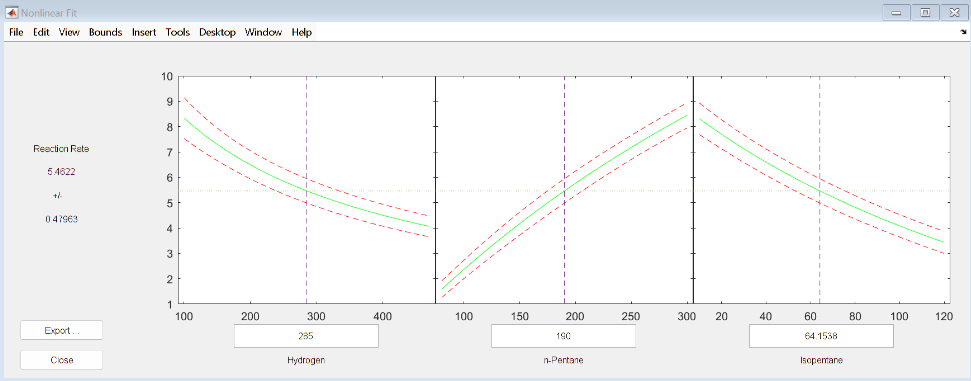
displays plots of the fitted response against each predictor, with the other predictors held
fixed. Dashed red curves show 95% simultaneous confidence bounds for the function. The fixed
values are displayed in the text boxes below each predictor axis. Change the fixed values by
entering new values or by dragging the vertical lines in the plots to new positions. When you
change the value of a predictor, the tool updates all plots to display the model at the new
point in the predictor space. Use the Export button to export specified variables to the
workspace.
Required Products
MATLAB®
Statistics and Machine Learning Toolbox™
Open the Nonlinear Regression Fitter Tool
At the MATLAB command prompt, enter
nlintool.
Examples
Perform nonlinear regression and display fitted model responses for different predictor values using the Nonlinear Regression Fitter tool.
Load the reaction kinetics data set. The observations in reactants are partial pressures of the three chemical reactants listed in xn. The corresponding reaction rates (responses) are stored in rate.
load reactionFit the Hougen-Watson model to the data using the initial model coefficient values in beta. Specify to show 99% confidence bounds and to label the plot axes.
nlintool(reactants,rate,@hougen,beta,Alpha=0.01,XName=xn,YName=yn)
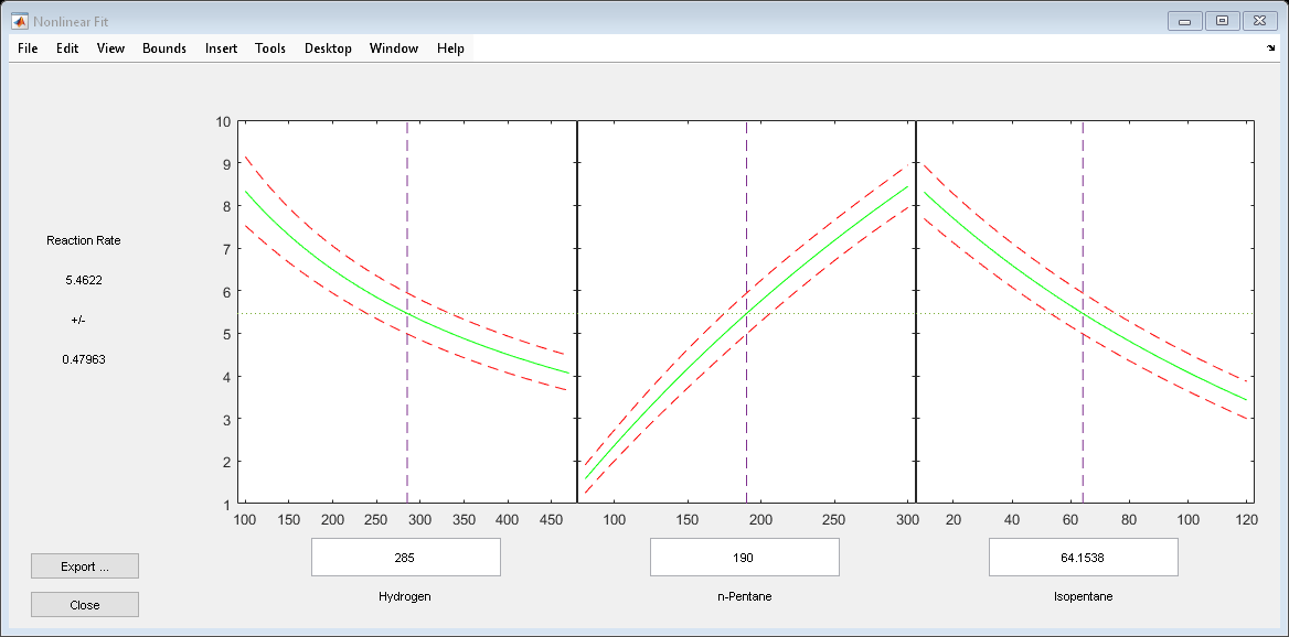
The tool displays plots of the fitted response against each predictor. The solid green curve shows the predicted response for that predictor when the other predictor values are fixed. You can change the fixed values by entering new values in the text boxes, or by dragging the vertical lines in the plots to new positions. When you change the value of a predictor the tool updates all plots to display the model at the new point in the predictor space. The dashed red lines indicate the 99% confidence bounds.
Related Examples
Programmatic Use
Tips
Use the Bounds menu in the tool window to select the type of confidence bounds: simultaneous or non-simultaneous, and curve or observation.
Simultaneous or Non-Simultaneous
Simultaneous (default) —
nlintoolcomputes confidence bounds for the curve of the response values using Scheffé's method. The range between the upper and lower confidence bounds contains the curve consisting of true response values with 95% confidence.Non-Simultaneous —
nlintoolcomputes confidence bounds for the response value at each observation. The confidence interval for a response value at a specific predictor value contains the true response value with 95% confidence.
With simultaneous bounds, the entire curve of true response values is within the bounds at high confidence. By contrast, non-simultaneous bounds require only the response value at a single predictor value to be within the bounds at high confidence. Therefore, simultaneous bounds are wider than non-simultaneous bounds.
Curve or Observation
A regression model for the predictor variables X and the response variable Y has the form
Y = f(X) + ε,
where f is a function of X and ε is a random noise term.
Curve (default) —
nlintoolplots confidence bounds for the fitted responses f(X).Observation —
nlintoolplots confidence bounds for the response observations Y.
The bounds for Y are wider than the bounds for f(X) because of the noise term.
If you do not want the plot to display confidence bounds, you can select No Bounds.
Version History
Introduced before R2006a