Partition Data Using Spectral Clustering
This topic provides an introduction to spectral clustering and an example that estimates the number of clusters and performs spectral clustering.
Introduction to Spectral Clustering
Spectral clustering is a graph-based algorithm for partitioning data points, or
observations, into k clusters. The Statistics and Machine Learning Toolbox™ function spectralcluster performs clustering on an input data matrix or on a
similarity matrix of a similarity graph derived from the data.
spectralcluster returns the cluster indices, a matrix
containing k eigenvectors of the Laplacian
matrix, and a vector of eigenvalues corresponding to the
eigenvectors.
spectralcluster requires you to specify the number of
clusters k. However, you can verify that your estimate for
k is correct by using one of these methods:
Count the number of zero eigenvalues of the Laplacian matrix. The multiplicity of the zero eigenvalues is an indicator of the number of clusters in your data.
Find the number of connected components in your similarity matrix by using the MATLAB® function
conncomp.
Algorithm Description
Spectral clustering is a graph-based algorithm for finding k arbitrarily shaped clusters in data. The technique involves representing the data in a low dimension. In the low dimension, clusters in the data are more widely separated, enabling you to use algorithms such as k-means or k-medoids clustering. This low dimension is based on the eigenvectors corresponding to the k smallest eigenvalues of a Laplacian matrix. A Laplacian matrix is one way of representing a similarity graph that models the local neighborhood relationships between data points as an undirected graph. The spectral clustering algorithm derives a similarity matrix of a similarity graph from your data, finds the Laplacian matrix, and uses the Laplacian matrix to find k eigenvectors for splitting the similarity graph into k partitions. You can use spectral clustering when you know the number of clusters, but the algorithm also provides a way to estimate the number of clusters in your data.
By default, the algorithm for spectralcluster computes the normalized random-walk Laplacian matrix
using the method described by Shi-Malik [1].
spectralcluster also supports the unnormalized Laplacian
matrix and the normalized symmetric Laplacian matrix which uses the Ng-Jordan-Weiss
method [2]. The
spectralcluster function implements clustering as
follows:
For each data point in
X, define a local neighborhood using either the radius search method or nearest neighbor method, as specified by the'SimilarityGraph'name-value pair argument (see Similarity Graph). Then, find the pairwise distances for all points i and j in the neighborhood.Convert the distances to similarity measures using the kernel transformation . The matrix S is the similarity matrix, and σ is the scale factor for the kernel, as specified using the
'KernelScale'name-value pair argument.Calculate the unnormalized Laplacian matrix L , the normalized random-walk Laplacian matrix Lrw, or the normalized symmetric Laplacian matrix Ls, depending on the value of the
'LaplacianNormalization'name-value pair argument.Create a matrix containing columns , where the columns are the k eigenvectors that correspond to the k smallest eigenvalues of the Laplacian matrix. If using Ls, normalize each row of V to have unit length.
Treating each row of V as a point, cluster the n points using k-means clustering (default) or k-medoids clustering, as specified by the
'ClusterMethod'name-value pair argument.Assign the original points in
Xto the same clusters as their corresponding rows in V.
Estimate Number of Clusters and Perform Spectral Clustering
This example demonstrates two approaches for performing spectral clustering.
The first approach estimates the number of clusters using the eigenvalues of the Laplacian matrix and performs spectral clustering on the data set.
The second approach estimates the number of clusters using the similarity graph and performs spectral clustering on the similarity matrix.
Generate Sample Data
Randomly generate a sample data set with three well-separated clusters, each containing 20 points.
rng('default'); % For reproducibility
n = 20;
X = [randn(n,2)*0.5+3;
    randn(n,2)*0.5;
    randn(n,2)*0.5-3];
Perform Spectral Clustering on Data
Estimate the number of clusters in the data by using the eigenvalues of the Laplacian matrix, and perform spectral clustering on the data set.
Compute the five smallest eigenvalues (in magnitude) of the Laplacian matrix by using the spectralcluster function. By default, the function uses the normalized random-walk Laplacian matrix.
[~,V_temp,D_temp] = spectralcluster(X,5)
V_temp = 60×5

   -0.2236   -0.0000   -0.0000    0.1534   -0.0000
   -0.2236   -0.0000   -0.0000   -0.3093    0.0000
   -0.2236   -0.0000   -0.0000    0.2225    0.0000
   -0.2236   -0.0000   -0.0000    0.1776   -0.0000
   -0.2236   -0.0000   -0.0000    0.1331    0.0000
   -0.2236   -0.0000   -0.0000    0.2176    0.0000
   -0.2236   -0.0000   -0.0000    0.1967    0.0000
   -0.2236   -0.0000   -0.0000   -0.0088    0.0000
   -0.2236   -0.0000   -0.0000   -0.2844   -0.0000
   -0.2236   -0.0000   -0.0000   -0.3275   -0.0000
   -0.2236   -0.0000   -0.0000    0.2176    0.0000
   -0.2236   -0.0000   -0.0000   -0.3291   -0.0000
   -0.2236   -0.0000   -0.0000   -0.2081   -0.0000
   -0.2236   -0.0000   -0.0000   -0.0571   -0.0000
   -0.2236   -0.0000   -0.0000   -0.2642   -0.0000
      ⋮
D_temp = 5×1

    0.0000
   -0.0000
   -0.0000
    0.0876
    0.1653
Only the first three eigenvalues are approximately zero. The number of zero eigenvalues is a good indicator of the number of connected components in a similarity graph and, therefore, is a good estimate of the number of clusters in your data. So, k=3 is a good estimate of the number of clusters in X.
Perform spectral clustering on observations by using the spectralcluster function. Specify k=3 clusters.
k = 3;
[idx1,V,D] = spectralcluster(X,k)
idx1 = 60×1

     1
     1
     1
     1
     1
     1
     1
     1
     1
     1
     1
     1
     1
     1
     1
      ⋮
V = 60×3

    0.2236   -0.0000   -0.0000
    0.2236   -0.0000   -0.0000
    0.2236   -0.0000   -0.0000
    0.2236   -0.0000   -0.0000
    0.2236   -0.0000   -0.0000
    0.2236   -0.0000   -0.0000
    0.2236   -0.0000   -0.0000
    0.2236   -0.0000   -0.0000
    0.2236   -0.0000   -0.0000
    0.2236   -0.0000   -0.0000
    0.2236   -0.0000   -0.0000
    0.2236   -0.0000   -0.0000
    0.2236   -0.0000   -0.0000
    0.2236   -0.0000   -0.0000
    0.2236   -0.0000   -0.0000
      ⋮
D = 3×1
10-16 ×

    0.6142
   -0.1814
   -0.3754
Elements of D correspond to the three smallest eigenvalues of the Laplacian matrix. The columns of V contain the eigenvectors corresponding to the eigenvalues in D. For well-separated clusters, the eigenvectors are indicator vectors. The eigenvectors have values of zero (or close to zero) for points that do not belong to a particular cluster, and nonzero values for points that belong to a particular cluster.
Visualize the result of clustering.
gscatter(X(:,1),X(:,2),idx1);
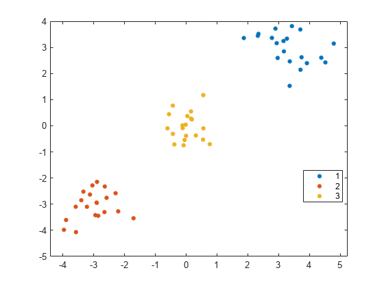
The spectralcluster function correctly identifies the three clusters in the data set.
Instead of using the spectralcluster function again, you can pass V_temp to the kmeans function to cluster the data points.
idx2 = kmeans(V_temp(:,1:3),3);
gscatter(X(:,1),X(:,2),idx2);

The order of cluster assignments in idx1 and idx2 is different even though the data points are clustered in the same way.
Perform Spectral Clustering on Similarity Matrix
Estimate the number of clusters using the similarity graph and perform spectral clustering on the similarity matrix.
Find the distance between each pair of observations in X by using the pdist and squareform functions with the default Euclidean distance metric.
dist_temp = pdist(X);
dist = squareform(dist_temp);
Construct the similarity matrix from the pairwise distance and confirm that the similarity matrix is symmetric.
S = exp(-dist.^2);
issymmetric(S)
ans = logical
   1
Limit the similarity values to 0.5 so that the similarity graph connects only points whose pairwise distances are smaller than the search radius.
S_eps = S;
S_eps(S_eps<0.5) = 0;
Create a graph object from S.
G_eps = graph(S_eps);
Visualize the similarity graph.
plot(G_eps)
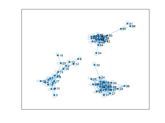
Identify the number of connected components in graph G_eps by using the unique and conncomp functions.
unique(conncomp(G_eps))
ans = 1×3

     1     2     3
The similarity graph shows three sets of connected components. The number of connected components in the similarity graph is a good estimate of the number of clusters in your data. Therefore, k=3 is a good choice for the number of clusters in X.
Perform spectral clustering on the similarity matrix derived from the data set X.
k = 3;
idx3 = spectralcluster(S_eps,k,'Distance','precomputed');
gscatter(X(:,1),X(:,2),idx3);
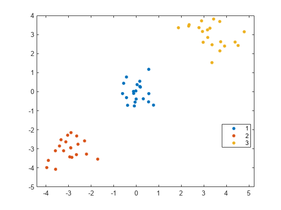
The spectralcluster function correctly identifies the three clusters in the data set.
References
[1] Shi, J., and J. Malik. “Normalized cuts and image segmentation.” IEEE Transactions on Pattern Analysis and Machine Intelligence. Vol. 22, 2000, pp. 888–905.
[2] Ng, A.Y., M. Jordan, and Y. Weiss. “On spectral clustering: Analysis and an algorithm.” In Proceedings of the Advances in Neural Information Processing Systems 14. MIT Press, 2001, pp. 849–856.
See Also
spectralcluster | pdist2 | pdist | squareform | adjacency | conncomp