templateNeuralNetwork

R2026b

Neural network template

Since R2026b

Syntax

t = templateNeuralNetwork

t = templateNeuralNetwork(Name=Value)

Description

t = templateNeuralNetwork returns a neural network template suitable for training a neural network classification or regression model. Specify t as a learner in one of the following functions:

testckfold — Compare the accuracy of two classification models through repeated cross-validation.
fitsemiself — Label data using a semi-supervised self-training method.
directforecaster — Fit a multistep forecasting model that uses a direct strategy in which a separate regression model is trained for each step of the forecasting horizon.

t = templateNeuralNetwork(Name=Value) creates a template with additional options specified by one or more name-value arguments. For example, you can adjust the number of outputs and the activation functions for the fully connected layers.

If you specify the type of model by using the Type name-value argument, then the display of t in the Command Window shows all configurable options as empty ([]), except those that you specify using name-value arguments. If you do not specify the type of model, then the display suppresses the empty options. During training, the software uses the default values for empty options.

example

Examples

collapse all

Compare Classification Accuracy of Neural Network Models

Open Live Script

Conduct a statistical test to assess whether a simpler neural network classifier has better accuracy than a more complex neural network classifier by using a 10-by-10 repeated cross-validation t test.

Load the fisheriris data set, which contains iris data including sepal length, sepal width, petal width, and species type. Specify the order of the iris species.

load fisheriris
tabulate(species)

       Value    Count   Percent
      setosa       50     33.33%
  versicolor       50     33.33%
   virginica       50     33.33%

classNames = ["setosa","versicolor","virginica"];

Create two neural network templates: one that uses a single fully connected layer with 10 outputs, and one that uses three fully connected layers with 30, 20, and 10 outputs, respectively. In both templates, standardize the numeric predictors.

simpleNet = templateNeuralNetwork(Standardize=true)

simpleNet = 
Fit template with properties:
    
         Method: 'NeuralNetwork'
           Type: ''

   Configurable Options:

    Standardize: 1

complexNet = templateNeuralNetwork(LayerSize=[30 20 10], ...
Standardize=true)

complexNet = 
Fit template with properties:
    
         Method: 'NeuralNetwork'
           Type: ''

   Configurable Options:

      LayerSize: [30 20 10]
    Standardize: 1

simpleNet and complexNet are neural network template objects.

Test the null hypothesis that the simpler model (simpleNet) is at most as accurate as the more complex model (complexNet) in terms of classification error. Conduct a 10-by-10 repeated cross-validation test, and return the p-value.

rng(0,"twister") % For reproducibility
[h,p] = testckfold(simpleNet,complexNet,meas,meas,species, ...
Alternative="greater",Test="10x10t",ClassNames=classNames)

h = logical
   0

p = 
0.3621

The p-value is approximately 0.33, which indicates to retain the null hypothesis that the simpler model is at most as accurate as the more complex model.

Create Direct Forecasting Model Using Custom Neural Network with Input Layer

This example uses:

Open Live Script

Create a direct forecasting model using a custom neural network with a complex architecture (that is, with a skip connection and an input layer). Specify the architecture using a dlnetwork (Deep Learning Toolbox) object in the call to the templateNeuralNetwork function, and then pass the template to directforecaster.

In general, you do not need to specify an input layer unless you want to use functionality provided by the input layer.

Load the sample file TemperatureData.csv, which contains average daily temperatures from January 2015 through July 2016. Read the file into a table. Observe the first eight observations in the table.

temperatures = readtable("TemperatureData.csv");
head(temperatures)

    Year       Month       Day    TemperatureF
    ____    ___________    ___    ____________

    2015    {'January'}     1          23     
    2015    {'January'}     2          31     
    2015    {'January'}     3          25     
    2015    {'January'}     4          39     
    2015    {'January'}     5          29     
    2015    {'January'}     6          12     
    2015    {'January'}     7          10     
    2015    {'January'}     8           4

For this example, use a subset of the temperature data that omits the first 100 observations.

Tbl = temperatures(101:end,:);

Create a datetime variable t that contains the year, month, and day information for each observation in Tbl. Then, use t to convert Tbl into a timetable.

numericMonth = month(datetime(Tbl.Month, ...
    InputFormat="MMMM",Locale="en_US"));
t = datetime(Tbl.Year,numericMonth,Tbl.Day);
Tbl.Time = t;
Tbl = table2timetable(Tbl);

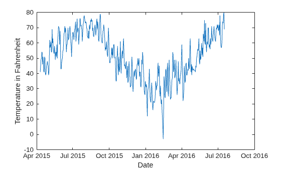
Plot the temperature values in Tbl over time.

plot(Tbl.Time,Tbl.TemperatureF)
xlabel("Date")
ylabel("Temperature in Fahrenheit")

Figure contains an axes object. The axes object with xlabel Date, ylabel Temperature in Fahrenheit contains an object of type line.

Create a template for a multilayer perceptron (MLP) neural network with a skip connection and a feature input layer.

First, determine the number of predictors to include in the feature input layer of the neural network using the helper function countDirectForecasterPredictors. Specify the options for direct forecasting and pass them, along with the training data Tbl, to the helper function. Note that all three of the predictors in Tbl (Year, Month, and Day) are leading predictors because their future values are known.

options = {"ResponseLags",1:7,"LeadingPredictors", ...
    1:3,"LeadingPredictorLags",{0:1,0:1,0:7},"CategoricalPredictors",2};
inputSize = countDirectForecasterPredictors(Tbl,"TemperatureF",options{:})

inputSize = 
41

Next, specify the neural network architecture.

net = dlnetwork;
layers = [
    featureInputLayer(inputSize)
    fullyConnectedLayer(12)
    reluLayer(Name="relu1")

    fullyConnectedLayer(12)

    additionLayer(2,Name="add2")
    reluLayer(Name="relu2")

    fullyConnectedLayer(12)
    additionLayer(2,Name="add3")
    reluLayer

    fullyConnectedLayer(1)];
net = addLayers(net,layers);
net = connectLayers(net,"relu1","add2/in2");
net = connectLayers(net,"relu2","add3/in2");

Finally, create a template for the neural network. Standardize the numeric predictors.

advancedNetTemplate = templateNeuralNetwork(Network=net,Standardize=true);

Create a full direct forecasting model by using the data in Tbl. Train the model using the neural network template. Specify the same options as those in options.

rng(0,"twister") % For reproducibility
Mdl = directforecaster(Tbl,"TemperatureF", ...
Learner=advancedNetTemplate, ...
ResponseLags=1:7,LeadingPredictors=1:3, ...
LeadingPredictorLags={0:1,0:1,0:7})

Mdl = 
  DirectForecaster

                  Horizon: 1
             ResponseLags: [1 2 3 4 5 6 7]
        LeadingPredictors: [1 2 3]
     LeadingPredictorLags: {[0 1]  [0 1]  [0 1 2 3 4 5 6 7]}
             ResponseName: 'TemperatureF'
           PredictorNames: {'Year'  'Month'  'Day'}
    CategoricalPredictors: 2
                 Learners: {[1×1 classreg.learning.regr.CompactRegressionNeuralNetwork]}
                   MaxLag: 7
          NumObservations: 465


  Properties, Methods

Mdl is a DirectForecaster model object with a CompactRegressionNeuralNetwork model object in its Learners property. If you use the forecast object function, Mdl uses the trained neural network model to forecast one step ahead.

You can display more information about the neural network by using the dlnetwork object function.

dlnetwork(Mdl.Learners{1})

ans = 
  dlnetwork with properties:

         Layers: [10×1 nnet.cnn.layer.Layer]
    Connections: [11×2 table]
     Learnables: [8×3 table]
          State: [0×3 table]
     InputNames: {'input'}
    OutputNames: {'fc_4'}
    Initialized: 1

  View summary with summary.

countDirectForecasterPredictors

The countDirectForecasterPredictors helper function takes a matrix, table, or timetable X, a response variable Y (either a numeric vector or a column name in X), and a cell array of direct forecasting options, and returns the number of predictors to include in a neural network feature input layer when you use directforecaster.

function inputSize = countDirectForecasterPredictors(X,Y,options)

% Set default values for lags and predictors
arguments
    X
    Y
    options.ResponseLags = 1;
    options.PredictorLags = 1;
    options.LeadingPredictors = [];
    options.LeadingPredictorLags = 0;
    options.CategoricalPredictors = [];
end

% Convert timetable to table
if istimetable(X)
    X = timetable2table(X,ConvertRowTimes=false);
end

% Remove response from table
if istable(X) && ~isnumeric(Y)
    X.(Y) = [];
end

% Count number of predictors in X
numPredictors = size(X,2);

% Find leading predictors and categorical predictors
leadingPredictorFlag = false(1,numPredictors);
leadingPredictorFlag(options.LeadingPredictors) = true;
categoricalPredictorFlag = false(1,numPredictors);
categoricalPredictorFlag(options.CategoricalPredictors) = true;

% Find predictors due to lagged leading and nonleading predictors
predictorLags = options.PredictorLags;
if isnumeric(predictorLags)
    predictorLags = repmat({predictorLags},1,sum(~leadingPredictorFlag));
end

leadPredictorLags = options.LeadingPredictorLags;
if isnumeric(leadPredictorLags)
    leadPredictorLags = repmat({leadPredictorLags},1,sum(leadingPredictorFlag));
end

lags = cell(1,numPredictors);
lags(1,leadingPredictorFlag) = leadPredictorLags;
lags(1,~leadingPredictorFlag) = predictorLags;

% Count number of predictors due to lagged response
inputSize = numel(options.ResponseLags);

% Count number of predictors after categorical encoding; include predictors
% due to lags
for ij = 1:numPredictors
    numExpandedFeatures = countPredictorsAfterCategoricalEncoding(X(:,ij), ...
        CategoricalPredictors=categoricalPredictorFlag(ij));
    inputSize = inputSize + numExpandedFeatures * numel(lags{ij});   
end

end

Name-Value Arguments

expand all

Specify optional pairs of arguments as Name1=Value1,...,NameN=ValueN, where Name is the argument name and Value is the corresponding value. Name-value arguments must appear after other arguments, but the order of the pairs does not matter.

Example: templateNeuralNetwork(LayerSizes=[10 10],Activations=["relu","tanh"]) creates a template for a neural network with two fully connected layers, each with 10 outputs. The first layer uses a rectified linear unit (ReLU) activation function, and the second uses a hyperbolic tangent activation function.

Classification Models and Regression Models

expand all

`Type` — Neural network model type
`"classification"` | `"regression"`

Neural network model type, specified as "classification" or "regression".

Value	Description
`"classification"`	Create a neural network learner template for classification. If you do not specify `Type` as `"classification"`, the fitting functions `testckfold` and `fitsemiself` set this value when you pass `t` to them.
`"regression"`	Create a neural network learner template for regression. If you do not specify `Type` as `"regression"`, the fitting function `directforecaster` sets this value when you pass `t` to it.

Example: Type="classification"

Data Types: char | string

`LayerSizes` — Sizes of fully connected layers
positive integer vector | `[]`

Sizes of the fully connected layers in the neural network model, specified as one of these values:

Positive integer vector — Element i of LayerSizes is the number of outputs in fully connected layer i of the neural network model. LayerSizes does not include the size of the final fully connected layer. For more information, see Classification Neural Network Structure and Regression Neural Network Structure.
[] — If you specify the neural network architecture using the Network argument, then LayerSizes must be [].

When Network is [], the default value of LayerSizes is 10; otherwise, the default value is [].

Example: LayerSizes=[100 25 10]

Data Types: single | double

`Activations` — Activation functions for fully connected layers
character vector | string scalar | string array | cell array of character vectors

Activation functions for the fully connected layers of the neural network model, specified as one of these values:

Character vector or string scalar — Use the specified activation function for each fully connected layer of the model. For classification models, the activation function for the final fully connected layer is always softmax and is not included in Activations. For more information, see Classification Neural Network Structure and Regression Neural Network Structure.
String array or cell array of character vectors — Use element i of Activations for fully connected layer i of the model.
"" — If you specify the neural network architecture using the Network argument, then Activations must be "".

Specify the activation functions using one or more of the values in the table below.

Value	Description
`"relu"`	Rectified linear unit (ReLU) function — Performs a threshold operation on each element of the input, where any value less than zero is set to zero, that is, $f (x) = {\begin{matrix} x, & x \geq 0 \\ 0, & x < 0 \end{matrix}$
`"tanh"`	Hyperbolic tangent (tanh) function — Applies the `tanh` function to each input element
`"sigmoid"`	Sigmoid function — Performs the following operation on each input element: $f (x) = \frac{1}{1 + e^{- x}}$
`"none"`	Identity function — Returns each input element without performing any transformation, that is, f(x) = x

When Network is [], the default value of Activations is "relu"; otherwise, the default value is [].

Example: Activations="sigmoid"

Example: Activations=["relu","tanh"]

Data Types: char | string | cell

`LayerWeightsInitializer` — Function to initialize fully connected layer weights
`"glorot"` | `"he"` | `""`

Function to initialize the fully connected layer weights, specified as one of these values:

"glorot" — Initialize the weights using the Glorot initializer [1] (also known as the Xavier initializer). For each layer, the Glorot initializer independently samples from a uniform distribution with zero mean and variance 2/(I+O), where I is the input size and O is the output size for the layer.
"he" — Initialize the weights using the He initializer [2]. For each layer, the He initializer samples from a normal distribution with zero mean and variance 2/I, where I is the input size for the layer.
"" — Initialize the weights using the initializers specified by the layers in the Network argument. If you specify the neural network architecture using the Network argument, do not change the value of the LayerWeightsInitializer argument.

When Network is [], the default value of LayerWeightsInitializer is "glorot"; otherwise, the default value is "".

Example: LayerWeightsInitializer="he"

Data Types: char | string

`LayerBiasesInitializer` — Type of initial fully connected layer biases
`"zeros"` | `"ones"` | `""`

Type of initial fully connected layer biases, specified as one of these values:

"zeros" — Initialize the biases using a vector of zeros.
"ones" — Initialize the biases using a vector of ones.
"" — Initialize the biases using the initializers specified by the layers in the Network argument. If you specify the neural network architecture using the Network argument, do not change the value of the LayerBiasesInitializer argument.

When Network is [], the default value of LayerBiasesInitializer is "zeros"; otherwise, the default value is "".

Example: LayerBiasesInitializer="ones"

Data Types: char | string

`Network` — Custom neural network architecture
`[]` (default) | layer array | `dlnetwork` object

Custom neural network architecture, specified as one of these values:

[] — Use the neural network architecture and layer configuration defined by the LayerSizes, Activations, LayerWeightsInitializer, and LayerBiasesInitializer arguments.
Layer array (requires Deep Learning Toolbox™) — Use the neural network architecture specified by the layer array. For a list of available layers, see List of Deep Learning Layers (Deep Learning Toolbox).
dlnetwork object (requires Deep Learning Toolbox) — Use the neural network architecture specified by the dlnetwork (Deep Learning Toolbox) object.

If you specify a network using a layer array or dlnetwork object, do not change the LayerSizes, Activations, LayerWeightsInitializer, and LayerBiasesInitializer arguments.

For layer array and dlnetwork input, the neural network architecture must support inputs where the categorical predictors are encoded as numeric vectors. To ensure this support, use one of the following approaches:

Specify a neural network architecture that does not have an input layer. In this case, the software automatically determines the network input size based on the training data and adds an input layer with the appropriate size. This approach is usually the easiest.
Specify a neural network architecture that has an input layer whose size is consistent with the training data after the categorical predictors are encoded. To count the number of predictors in tabular data after the categorical variables are encoded, use the countPredictorsAfterCategoricalEncoding function. Follow this approach when you want to use functionality provided by input layers.
If you standardize the predictors using the Standardize argument, then the input layer of the network must not perform normalization.

`Lambda` — Regularization term strength
`0` (default) | nonnegative scalar

Regularization term strength, specified as a nonnegative scalar. The software composes the objective function for minimization from the loss function (cross-entropy for classification and mean squared error for regression) and the ridge (L2) penalty term.

Example: Lambda=1e-4

Data Types: single | double

`Standardize` — Flag to standardize predictor data
`false` or `0` (default) | `true` or `1`

Flag to standardize the predictor data, specified as a numeric or logical 0 (false) or 1 (true). If you set Standardize to true, then the software centers and scales each numeric predictor variable by the corresponding column mean and standard deviation. The software does not standardize categorical predictors.

If you specify the neural network architecture using the Network argument, and you want to standardize the predictors using the Standardize argument, the input layer of the network must not perform normalization.

Example: Standardize=true

Data Types: single | double | logical

Regression Models Only

expand all

`StandardizeResponses` — Flag to standardize response data
`false` or `0` (default) | `true` or `1`

Flag to standardize the response data before fitting the model, specified as a numeric or logical 0 (false) or 1 (true). If you set StandardizeResponses to true, then the software centers and scales each response variable by the corresponding column mean and standard deviation.

Example: StandardizeResponses=true

Data Types: single | double | logical

Convergence Control

expand all

`Verbose` — Verbosity level
`0` (default) | `1`

Verbosity level, specified as 0 or 1. The Verbose name-value argument controls the amount of diagnostic information that the software displays at the command line.

Value	Description
`0`	`templateNeuralNetwork` does not display diagnostic information.
`1`	`templateNeuralNetwork` periodically displays diagnostic information.

Example: Verbose=1

Data Types: single | double

`VerboseFrequency` — Frequency of verbose printing
`1` (default) | positive integer scalar

Frequency of verbose printing, which is the number of iterations between printing diagnostic information at the command line, specified as a positive integer scalar. A value of 1 indicates to print diagnostic information at every iteration.

Note

To use this name-value argument, you must set Verbose to 1.

Example: VerboseFrequency=5

Data Types: single | double

`InitialStepSize` — Initial step size
`[]` (default) | positive scalar | `"auto"`

Initial step size, specified as a positive scalar or "auto". By default, the software does not use the initial step size to determine the initial Hessian approximation used in training the model (see Training Solver). However, if you specify an initial step size ${‖ s_{0} ‖}_{\infty}$ , then the initial inverse-Hessian approximation is $\frac{{‖ s_{0} ‖}_{\infty}}{{‖ \nabla ℒ_{0} ‖}_{\infty}} I$ . $\nabla ℒ_{0}$ is the initial gradient vector, and $I$ is the identity matrix.

To have the software determine an initial step size automatically, specify the value as "auto". In this case, the software determines the initial step size by using ${‖ s_{0} ‖}_{\infty} = 0.5 {‖ η_{0} ‖}_{\infty} + 0.1$ . $s_{0}$ is the initial step vector, and $η_{0}$ is the vector of unconstrained initial weights and biases.

Example: InitialStepSize="auto"

Data Types: single | double | char | string

`IterationLimit` — Maximum number of training iterations
`1e3` (default) | positive integer scalar

Maximum number of training iterations, specified as a positive integer scalar.

The software returns a trained model regardless of whether the training routine successfully converges.

Example: IterationLimit=1e8

Data Types: single | double

`GradientTolerance` — Relative gradient tolerance
`1e-6` (default) | nonnegative scalar

Relative gradient tolerance, specified as a nonnegative scalar.

Let $ℒ_{t}$ be the loss function at training iteration t, $\nabla ℒ_{t}$ be the gradient of the loss function with respect to the weights and biases at iteration t, and $\nabla ℒ_{0}$ be the gradient of the loss function at an initial point. If $\max | \nabla ℒ_{t} | \leq a \cdot GradientTolerance$ , where $a = \max (1, \min | ℒ_{t} |, \max | \nabla ℒ_{0} |)$ , then the training process terminates.

Example: GradientTolerance=1e-5

Data Types: single | double

`LossTolerance` — Loss tolerance
`1e-6` (default) | nonnegative scalar

Loss tolerance, specified as a nonnegative scalar.

If the function loss at some iteration is smaller than LossTolerance, then the training process terminates.

Example: LossTolerance=1e-8

Data Types: single | double

`StepTolerance` — Step size tolerance
`1e-6` (default) | nonnegative scalar

Step size tolerance, specified as a nonnegative scalar.

If the step size at some iteration is smaller than StepTolerance, then the training process terminates.

Example: StepTolerance=1e-4

Data Types: single | double

Output Arguments

collapse all

`t` — Neural network learner template
template object

Neural network learner template suitable for training neural network classification or regression models, returned as a template object. During training, the software uses default values for empty options.

More About

collapse all

Classification Neural Network Structure

The default neural network classifier has the following layer structure.

Structure	Description
	Input — This layer corresponds to the predictor data.
	First fully connected layer — This layer has 10 outputs by default. You can widen the layer or add more fully connected layers to the network by specifying the `LayerSizes` name-value argument. You can find the weights and biases for this layer in the `Mdl.LayerWeights{1}` and `Mdl.LayerBiases{1}` properties of the model `Mdl`, respectively.
	ReLU activation function — The software applies this activation function to the first fully connected layer. You can change the activation function by specifying the `Activations` name-value argument.
	Final fully connected layer — This layer has K outputs, where K is the number of classes in the response variable. You can find the weights and biases for this layer in the `Mdl.LayerWeights{end}` and `Mdl.LayerBiases{end}` properties of the model `Mdl`, respectively.
	Softmax function (for both binary and multiclass classification) — The software applies this activation function to the final fully connected layer. The function takes each input x_i and returns the following, where K is the number of classes in the response variable: $f (x_{i}) = \frac{\exp (x_{i})}{\sum_{j = 1}^{K} \exp (x_{j})} .$ The results correspond to the predicted classification scores (or posterior probabilities).
	Output — This layer corresponds to the predicted class labels.

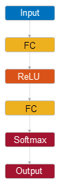
For an example that shows how a neural network classifier with this layer structure returns predictions, see Predict Using Layer Structure of Neural Network Classifier.

To specify a custom neural network architecture, use the Network name-value argument.

Regression Neural Network Structure

The default neural network regression model has the following layer structure.

Structure	Description
	Input — This layer corresponds to the predictor data.
	First fully connected layer — This layer has 10 outputs by default. You can widen the layer or add more fully connected layers to the network by specifying the `LayerSizes` name-value argument. You can find the weights and biases for this layer in the `Mdl.LayerWeights{1}` and `Mdl.LayerBiases{1}` properties of the model `Mdl`, respectively.
	ReLU activation function — The software applies this activation function to the first fully connected layer. You can change the activation function by specifying the `Activations` name-value argument.
	Final fully connected layer — This layer has one output for each response variable. You can find the weights and biases for this layer in the `Mdl.LayerWeights{end}` and `Mdl.LayerBiases{end}` properties of the model `Mdl`, respectively.
	Output — This layer corresponds to the predicted response values.

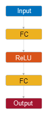
For an example that shows how a regression neural network model with this layer structure returns predictions, see Predict Using Layer Structure of Regression Neural Network Model.

To specify a custom neural network architecture, use the Network name-value argument.

Training Solver

The software uses a limited-memory Broyden–Fletcher–Goldfarb–Shanno quasi-Newton algorithm (LBFGS) [3] as its loss function minimization technique, where the software minimizes the cross-entropy loss for classification and the mean squared error (MSE) for regression. The LBFGS solver uses a standard line-search method with an approximation to the Hessian.

References

[1] Glorot, Xavier, and Yoshua Bengio. “Understanding the Difficulty of Training Deep Feedforward Neural Networks.” In Proceedings of the 13th international conference on artificial intelligence and statistics, pp. 249–256, 2010.

[2] He, Kaiming, Xiangyu Zhang, Shaoqing Ren, and Jian Sun. “Delving Deep into Rectifiers: Surpassing Human-Level Performance on ImageNet Classification.” In Proceedings of the IEEE international conference on computer vision, pp. 1026–1034, 2015.

[3] Nocedal, J., and S. J. Wright. Numerical Optimization, 2nd ed., New York: Springer, 2006.

Version History

Introduced in R2026b

templateNeuralNetwork

Syntax

Description

Examples

Compare Classification Accuracy of Neural Network Models

Create Direct Forecasting Model Using Custom Neural Network with Input Layer

Name-Value Arguments

Classification Models and Regression Models

Type — Neural network model type "classification" | "regression"

LayerSizes — Sizes of fully connected layers positive integer vector | []

Activations — Activation functions for fully connected layers character vector | string scalar | string array | cell array of character vectors

LayerWeightsInitializer — Function to initialize fully connected layer weights "glorot" | "he" | ""

LayerBiasesInitializer — Type of initial fully connected layer biases "zeros" | "ones" | ""

Network — Custom neural network architecture [] (default) | layer array | dlnetwork object

Lambda — Regularization term strength 0 (default) | nonnegative scalar

Standardize — Flag to standardize predictor data false or 0 (default) | true or 1

Regression Models Only

StandardizeResponses — Flag to standardize response data false or 0 (default) | true or 1

Convergence Control

Verbose — Verbosity level 0 (default) | 1

VerboseFrequency — Frequency of verbose printing 1 (default) | positive integer scalar

InitialStepSize — Initial step size [] (default) | positive scalar | "auto"

IterationLimit — Maximum number of training iterations 1e3 (default) | positive integer scalar

GradientTolerance — Relative gradient tolerance 1e-6 (default) | nonnegative scalar

LossTolerance — Loss tolerance 1e-6 (default) | nonnegative scalar

StepTolerance — Step size tolerance 1e-6 (default) | nonnegative scalar

Output Arguments

t — Neural network learner template template object

More About

Classification Neural Network Structure

Regression Neural Network Structure

Training Solver

References

Version History

See Also

`Type` — Neural network model type
`"classification"` | `"regression"`

`LayerSizes` — Sizes of fully connected layers
positive integer vector | `[]`

`Activations` — Activation functions for fully connected layers
character vector | string scalar | string array | cell array of character vectors

`LayerWeightsInitializer` — Function to initialize fully connected layer weights
`"glorot"` | `"he"` | `""`

`LayerBiasesInitializer` — Type of initial fully connected layer biases
`"zeros"` | `"ones"` | `""`

`Network` — Custom neural network architecture
`[]` (default) | layer array | `dlnetwork` object

`Lambda` — Regularization term strength
`0` (default) | nonnegative scalar

`Standardize` — Flag to standardize predictor data
`false` or `0` (default) | `true` or `1`

`StandardizeResponses` — Flag to standardize response data
`false` or `0` (default) | `true` or `1`

`Verbose` — Verbosity level
`0` (default) | `1`

`VerboseFrequency` — Frequency of verbose printing
`1` (default) | positive integer scalar

`InitialStepSize` — Initial step size
`[]` (default) | positive scalar | `"auto"`

`IterationLimit` — Maximum number of training iterations
`1e3` (default) | positive integer scalar

`GradientTolerance` — Relative gradient tolerance
`1e-6` (default) | nonnegative scalar

`LossTolerance` — Loss tolerance
`1e-6` (default) | nonnegative scalar

`StepTolerance` — Step size tolerance
`1e-6` (default) | nonnegative scalar

`t` — Neural network learner template
template object