directforecaster
Description
DirectForecaster is a multistep forecasting model that uses a
direct strategy in which a separate regression model is trained for each step of the
forecasting horizon. For more information, see Direct Forecasting. Use the directforecaster function to train a
DirectForecaster model with regularly sampled time series
data.
You can use lagged and leading predictors to train the direct forecasting model.
directforecaster creates the appropriate predictors when you specify
the following:
Leading exogenous predictors (
LeadingPredictors)Lag values of the leading exogenous predictors (
LeadingPredictorLags)Lag values of the nonleading exogenous predictors (
PredictorLags)Lag values of the response (
ResponseLags)
For more information, see Forecasting Data.
After creating a DirectForecaster object, you can see how the model
performs on observed test data by using the loss and predict object
functions. You can then use the model to forecast at time steps beyond the available data by
using the forecast object
function.
Creation
Syntax
Description
Mdl = directforecaster(Tbl,ResponseVarName)Mdl using the regularly sampled
data in Tbl and the response in variable
ResponseVarName in Tbl. The function treats
all variables in Tbl other than ResponseVarName
as exogenous predictor variables.
By default, the resulting Mdl object contains one regression
model, with a time horizon of one step ahead. directforecaster uses a
lag value of 1 to create predictors from the exogenous predictors and
the response variable.
Mdl = directforecaster(__,Name=Value)Horizon=[1
3 5].
Input Arguments
Name-Value Arguments
Output Arguments
Properties
Object Functions
compact | Reduce size of direct forecasting model |
crossval | Cross-validate direct forecasting model |
loss | Loss at each horizon step |
predict | Predict response at time steps in observed test data |
forecast | Forecast response at time steps beyond available data |
preparedPredictors | Obtain prepared data used for training or testing in direct forecasting |
Examples
Calculate the test set mean squared error (MSE) of a direct forecasting model.
Load the sample file TemperatureData.csv, which contains average daily temperatures from January 2015 through July 2016. Read the file into a table. Observe the first eight observations in the table.
temperatures = readtable("TemperatureData.csv");
head(temperatures)
Year Month Day TemperatureF
____ ___________ ___ ____________
2015 {'January'} 1 23
2015 {'January'} 2 31
2015 {'January'} 3 25
2015 {'January'} 4 39
2015 {'January'} 5 29
2015 {'January'} 6 12
2015 {'January'} 7 10
2015 {'January'} 8 4
For this example, use a subset of the temperature data that omits the first 100 observations.
Tbl = temperatures(101:end,:);
Create a datetime variable t that contains the year, month, and day information for each observation in Tbl. Then, use t to convert Tbl into a timetable.
numericMonth = month(datetime(Tbl.Month, ...
    InputFormat="MMMM",Locale="en_US"));
t = datetime(Tbl.Year,numericMonth,Tbl.Day);
Tbl.Time = t;
Tbl = table2timetable(Tbl);
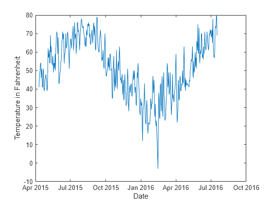
Plot the temperature values in Tbl over time.
plot(Tbl.Time,Tbl.TemperatureF)
xlabel("Date")
ylabel("Temperature in Fahrenheit")
Partition the temperature data into training and test sets by using tspartition. Reserve 20% of the observations for testing.
partition = tspartition(size(Tbl,1),"Holdout",0.20);
trainingTbl = Tbl(training(partition),:);
testTbl = Tbl(test(partition),:);
Create a full direct forecasting model by using the data in trainingTbl. Train the model using a decision tree learner. All three of the predictors (Year, Month, and Day) are leading predictors because their future values are known. To create new predictors by shifting the leading predictor and response variables backward in time, specify the leading predictor lags and the response variable lags.
Mdl = directforecaster(trainingTbl,"TemperatureF", ...
    Learner="tree", ...
    LeadingPredictors="all",LeadingPredictorLags={0:1,0:1,0:7}, ...
    ResponseLags=1:7)
Mdl =
  DirectForecaster

                  Horizon: 1
             ResponseLags: [1 2 3 4 5 6 7]
        LeadingPredictors: [1 2 3]
     LeadingPredictorLags: {[0 1]  [0 1]  [0 1 2 3 4 5 6 7]}
             ResponseName: 'TemperatureF'
           PredictorNames: {'Year'  'Month'  'Day'}
    CategoricalPredictors: 2
                 Learners: {[1×1 classreg.learning.regr.CompactRegressionTree]}
                   MaxLag: 7
          NumObservations: 372


  Properties, Methods
Mdl is a DirectForecaster model object. By default, the horizon is one step ahead. That is, Mdl predicts a value that is one step into the future.
Calculate the test set MSE. Smaller MSE values indicate better performance.
testMSE = loss(Mdl,testTbl)
testMSE =
61.0849
After creating a DirectForecaster object, see how the model performs on observed test data by using the predict object function. Then use the model to forecast at time steps beyond the available data by using the forecast object function.
Load the sample file TemperatureData.csv, which contains average daily temperatures from January 2015 through July 2016. Read the file into a table. Observe the first eight observations in the table.
temperatures = readtable("TemperatureData.csv");
head(temperatures)
Year Month Day TemperatureF
____ ___________ ___ ____________
2015 {'January'} 1 23
2015 {'January'} 2 31
2015 {'January'} 3 25
2015 {'January'} 4 39
2015 {'January'} 5 29
2015 {'January'} 6 12
2015 {'January'} 7 10
2015 {'January'} 8 4
For this example, use a subset of the temperature data that omits the first 100 observations.
Tbl = temperatures(101:end,:);
Create a datetime variable t that contains the year, month, and day information for each observation in Tbl. Then, use t to convert Tbl into a timetable.
numericMonth = month(datetime(Tbl.Month, ...
    InputFormat="MMMM",Locale="en_US"));
t = datetime(Tbl.Year,numericMonth,Tbl.Day);
Tbl.Time = t;
Tbl = table2timetable(Tbl);
Plot the temperature values in Tbl over time.
plot(Tbl.Time,Tbl.TemperatureF)
xlabel("Date")
ylabel("Temperature in Fahrenheit")

Partition the temperature data into training and test sets by using tspartition. Reserve 20% of the observations for testing.
partition = tspartition(size(Tbl,1),"Holdout",0.20);
trainingTbl = Tbl(training(partition),:);
testTbl = Tbl(test(partition),:);
Create a full direct forecasting model by using the data in trainingTbl. Train the model using a decision tree learner. All three of the predictors (Year, Month, and Day) are leading predictors because their future values are known. To create new predictors by shifting the leading predictor and response variables backward in time, specify the leading predictor lags and the response variable lags.
Mdl = directforecaster(trainingTbl,"TemperatureF", ...
    Learner="tree", ...
    LeadingPredictors="all",LeadingPredictorLags={0:1,0:1,0:7}, ...
    ResponseLags=1:7)
Mdl =
  DirectForecaster

                  Horizon: 1
             ResponseLags: [1 2 3 4 5 6 7]
        LeadingPredictors: [1 2 3]
     LeadingPredictorLags: {[0 1]  [0 1]  [0 1 2 3 4 5 6 7]}
             ResponseName: 'TemperatureF'
           PredictorNames: {'Year'  'Month'  'Day'}
    CategoricalPredictors: 2
                 Learners: {[1×1 classreg.learning.regr.CompactRegressionTree]}
                   MaxLag: 7
          NumObservations: 372


  Properties, Methods
Mdl is a DirectForecaster model object. By default, the horizon is one step ahead. That is, Mdl predicts a value that is one step into the future.
For each test set observation, predict the temperature value using Mdl.
predictedY = predict(Mdl,testTbl)
predictedY=93×1 timetable
       Time        TemperatureF_Step1
    ___________    __________________

    16-Apr-2016          49.398
    17-Apr-2016          39.419
    18-Apr-2016          39.419
    19-Apr-2016          45.333
    20-Apr-2016          35.867
    21-Apr-2016          34.222
    22-Apr-2016          45.333
    23-Apr-2016          66.392
    24-Apr-2016          44.111
    25-Apr-2016              49
    26-Apr-2016              49
    27-Apr-2016          34.222
    28-Apr-2016          43.333
    29-Apr-2016          34.222
    30-Apr-2016          34.222
    01-May-2016          34.222
      ⋮
Plot the true response values and the predicted response values for the test set observations.
plot(testTbl.Time,testTbl.TemperatureF)
hold on
plot(predictedY.Time,predictedY.TemperatureF_Step1,"--")
hold off
legend("True","Predicted",Location="southeast")
xlabel("Date")
ylabel("Temperature in Fahrenheit")
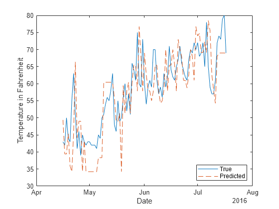
Overall, the direct forecasting model is able to predict the trend in temperatures.
Retrain the direct forecasting model using the training and test data. To forecast temperatures one week beyond the available data, specify the horizon steps as one to seven steps ahead.
finalMdl = directforecaster(Tbl,"TemperatureF", ...
    Learner="tree", ...
    LeadingPredictors="all",LeadingPredictorLags={0:1,0:1,0:7}, ...
    ResponseLags=1:7,Horizon=1:7)
finalMdl =
  DirectForecaster

                  Horizon: [1 2 3 4 5 6 7]
             ResponseLags: [1 2 3 4 5 6 7]
        LeadingPredictors: [1 2 3]
     LeadingPredictorLags: {[0 1]  [0 1]  [0 1 2 3 4 5 6 7]}
             ResponseName: 'TemperatureF'
           PredictorNames: {'Year'  'Month'  'Day'}
    CategoricalPredictors: 2
                 Learners: {7×1 cell}
                   MaxLag: 7
          NumObservations: 465


  Properties, Methods
finalMdl is a DirectForecaster model object that consists of seven regression models: finalMdl.Learners{1}, which predicts one step into the future; finalMdl.Learners{2}, which predicts two steps into the future; and so on.
Because finalMdl uses the unshifted values of the leading predictors Year, Month, and Day as predictor values, you must specify these values for the specified horizon steps in the call to forecast. For the week after the last available observation in Tbl, create a timetable forecastData with the year, month, and day values.
forecastTime = Tbl.Time(end,:)+1:Tbl.Time(end,:)+7;
forecastYear = year(forecastTime);
forecastMonth = month(forecastTime,"name");
forecastDay = day(forecastTime);
forecastData = timetable(forecastTime',forecastYear', ...
    forecastMonth',forecastDay',VariableNames=["Year","Month","Day"])
forecastData=7×3 timetable
       Time        Year     Month      Day
    ___________    ____    ________    ___

    18-Jul-2016    2016    {'July'}    18
    19-Jul-2016    2016    {'July'}    19
    20-Jul-2016    2016    {'July'}    20
    21-Jul-2016    2016    {'July'}    21
    22-Jul-2016    2016    {'July'}    22
    23-Jul-2016    2016    {'July'}    23
    24-Jul-2016    2016    {'July'}    24
Forecast the temperature at each horizon step using finalMdl.
forecastY = forecast(finalMdl,Tbl,LeadingData=forecastData)
forecastY=7×1 timetable
       Time        TemperatureF
    ___________    ____________

    18-Jul-2016       62.375
    19-Jul-2016         64.5
    20-Jul-2016       66.889
    21-Jul-2016       66.889
    22-Jul-2016         70.5
    23-Jul-2016        74.25
    24-Jul-2016        74.25
Plot the observed temperatures for the test set data and the forecast temperatures.
plot(testTbl.Time,testTbl.TemperatureF)
hold on
plot([testTbl.Time(end);forecastY.Time], ...
    [testTbl.TemperatureF(end);forecastY.TemperatureF],"--")
hold off
legend("Observed Data","Forecast Data", ...
    Location="southeast")
xlabel("Date")
ylabel("Temperature in Fahrenheit")

When you perform direct forecasting using directforecaster, the function creates lagged and leading predictors from the training data before fitting a DirectForecaster model. Similarly, the loss and predict object functions reformat the test data before computing loss and prediction values, respectively.
This example shows how to access the prepared predictor data used by direct forecasting models for training and testing.
Load the sample file TemperatureData.csv, which contains average daily temperatures from January 2015 through July 2016. Read the file into a table. Observe the first eight observations in the table.
temperatures = readtable("TemperatureData.csv");
head(temperatures)
Year Month Day TemperatureF
____ ___________ ___ ____________
2015 {'January'} 1 23
2015 {'January'} 2 31
2015 {'January'} 3 25
2015 {'January'} 4 39
2015 {'January'} 5 29
2015 {'January'} 6 12
2015 {'January'} 7 10
2015 {'January'} 8 4
For this example, use a subset of the temperature data that omits the first 100 observations.
Tbl = temperatures(101:end,:);
Create a datetime variable t that contains the year, month, and day information for each observation in Tbl. Then, use t to convert Tbl into a timetable.
numericMonth = month(datetime(Tbl.Month, ...
    InputFormat="MMMM",Locale="en_US"));
t = datetime(Tbl.Year,numericMonth,Tbl.Day);
Tbl.Time = t;
Tbl = table2timetable(Tbl);
Plot the temperature values in Tbl over time.
plot(Tbl.Time,Tbl.TemperatureF)
xlabel("Date")
ylabel("Temperature in Fahrenheit")

Partition the temperature data into training and test sets by using tspartition. Reserve 20% of the observations for testing.
partition = tspartition(size(Tbl,1),"Holdout",0.20);
trainingTbl = Tbl(training(partition),:);
testTbl = Tbl(test(partition),:);
Create a full direct forecasting model by using the data in trainingTbl. Specify the horizon steps as one to seven steps ahead. Train a model at each horizon step using a boosted ensemble of trees. All three of the predictors (Year, Month, and Day) are leading predictors because their future values are known.
To create new predictors by shifting the leading predictor and response variables backward in time, specify the leading predictor lags and the response variable lags. For this example, use the following as predictors values: the current and previous Year values, the current and previous Month values, the current and previous seven Day values, and the previous seven TemperatureF values.
Mdl = directforecaster(trainingTbl,"TemperatureF", ...
    Horizon=1:7,LeadingPredictors="all", ...
    LeadingPredictorLags={0:1,0:1,0:7}, ...
    ResponseLags=1:7)
Mdl =
  DirectForecaster

                  Horizon: [1 2 3 4 5 6 7]
             ResponseLags: [1 2 3 4 5 6 7]
        LeadingPredictors: [1 2 3]
     LeadingPredictorLags: {[0 1]  [0 1]  [0 1 2 3 4 5 6 7]}
             ResponseName: 'TemperatureF'
           PredictorNames: {'Year'  'Month'  'Day'}
    CategoricalPredictors: 2
                 Learners: {7×1 cell}
                   MaxLag: 7
          NumObservations: 372


  Properties, Methods
Mdl is a DirectForecaster model object. Mdl consists of seven regression models: Mdl.Learners{1}, which predicts one step into the future; Mdl.Learners{2}, which predicts two steps into the future; and so on.
Compare the first and seventh regression models in Mdl.
Mdl.Learners{1}ans =
CompactRegressionEnsemble
PredictorNames: {1×19 cell}
ResponseName: 'TemperatureF_Step1'
CategoricalPredictors: [10 11]
ResponseTransform: 'none'
NumTrained: 100
Properties, Methods
Mdl.Learners{7}ans =
CompactRegressionEnsemble
PredictorNames: {1×19 cell}
ResponseName: 'TemperatureF_Step7'
CategoricalPredictors: [10 11]
ResponseTransform: 'none'
NumTrained: 100
Properties, Methods
The regression models in Mdl are all CompactRegressionEnsemble objects. Because the models are compact, they do not include the predictor data used to train them.
To see the data used to train the regression models in Mdl, use the preparedPredictors object function.
Observe the prepared predictor data used to train Mdl.Learners{1}. By default, preparedPredictors returns the prepared predictor data used at horizon step Mdl.Horizon(1), which in this case is one step ahead.
prepTrainingTbl1 = preparedPredictors(Mdl,trainingTbl)
prepTrainingTbl1=372×19 timetable
       Time        TemperatureF_Lag1    TemperatureF_Lag2    TemperatureF_Lag3    TemperatureF_Lag4    TemperatureF_Lag5    TemperatureF_Lag6    TemperatureF_Lag7    Year_Step1    Year_Lag1    Month_Step1    Month_Lag1    Day_Step1    Day_Lag1    Day_Lag2    Day_Lag3    Day_Lag4    Day_Lag5    Day_Lag6    Day_Lag7
    ___________    _________________    _________________    _________________    _________________    _________________    _________________    _________________    __________    _________    ___________    __________    _________    ________    ________    ________    ________    ________    ________    ________

    10-Apr-2015           NaN                  NaN                  NaN                  NaN                  NaN                  NaN                  NaN              2015          NaN        {'April'}     {0×0 char}       10          NaN         NaN         NaN         NaN         NaN         NaN         NaN
    11-Apr-2015            41                  NaN                  NaN                  NaN                  NaN                  NaN                  NaN              2015         2015        {'April'}     {'April' }       11           10         NaN         NaN         NaN         NaN         NaN         NaN
    12-Apr-2015            45                   41                  NaN                  NaN                  NaN                  NaN                  NaN              2015         2015        {'April'}     {'April' }       12           11          10         NaN         NaN         NaN         NaN         NaN
    13-Apr-2015            49                   45                   41                  NaN                  NaN                  NaN                  NaN              2015         2015        {'April'}     {'April' }       13           12          11          10         NaN         NaN         NaN         NaN
    14-Apr-2015            50                   49                   45                   41                  NaN                  NaN                  NaN              2015         2015        {'April'}     {'April' }       14           13          12          11          10         NaN         NaN         NaN
    15-Apr-2015            54                   50                   49                   45                   41                  NaN                  NaN              2015         2015        {'April'}     {'April' }       15           14          13          12          11          10         NaN         NaN
    16-Apr-2015            54                   54                   50                   49                   45                   41                  NaN              2015         2015        {'April'}     {'April' }       16           15          14          13          12          11          10         NaN
    17-Apr-2015            46                   54                   54                   50                   49                   45                   41              2015         2015        {'April'}     {'April' }       17           16          15          14          13          12          11          10
    18-Apr-2015            51                   46                   54                   54                   50                   49                   45              2015         2015        {'April'}     {'April' }       18           17          16          15          14          13          12          11
    19-Apr-2015            47                   51                   46                   54                   54                   50                   49              2015         2015        {'April'}     {'April' }       19           18          17          16          15          14          13          12
    20-Apr-2015            41                   47                   51                   46                   54                   54                   50              2015         2015        {'April'}     {'April' }       20           19          18          17          16          15          14          13
    21-Apr-2015            41                   41                   47                   51                   46                   54                   54              2015         2015        {'April'}     {'April' }       21           20          19          18          17          16          15          14
    22-Apr-2015            51                   41                   41                   47                   51                   46                   54              2015         2015        {'April'}     {'April' }       22           21          20          19          18          17          16          15
    23-Apr-2015            50                   51                   41                   41                   47                   51                   46              2015         2015        {'April'}     {'April' }       23           22          21          20          19          18          17          16
    24-Apr-2015            40                   50                   51                   41                   41                   47                   51              2015         2015        {'April'}     {'April' }       24           23          22          21          20          19          18          17
    25-Apr-2015            39                   40                   50                   51                   41                   41                   47              2015         2015        {'April'}     {'April' }       25           24          23          22          21          20          19          18
      ⋮
prepTrainingTbl1 contains lagged predictors (with Lag in their names) and leading predictors (with Step in their names). The table contains missing values due to the creation of these prepared predictors. For example, TemperatureF_Lag1 contains a missing value at time 10-Apr-2015 because the temperature at time 09-Apr-2015 is not known.
Observe the prepared predictor data used to train Mdl.Learners{7}.
prepTrainingTbl7 = preparedPredictors(Mdl,trainingTbl, ...
HorizonStep=7)prepTrainingTbl7=372×19 timetable
Time TemperatureF_Lag1 TemperatureF_Lag2 TemperatureF_Lag3 TemperatureF_Lag4 TemperatureF_Lag5 TemperatureF_Lag6 TemperatureF_Lag7 Year_Step7 Year_Step6 Month_Step7 Month_Step6 Day_Step7 Day_Step6 Day_Step5 Day_Step4 Day_Step3 Day_Step2 Day_Step1 Day_Lag1
___________ _________________ _________________ _________________ _________________ _________________ _________________ _________________ __________ __________ ___________ ___________ _________ _________ _________ _________ _________ _________ _________ ________
10-Apr-2015 NaN NaN NaN NaN NaN NaN NaN 2015 NaN {'April'} {0×0 char} 10 NaN NaN NaN NaN NaN NaN NaN
11-Apr-2015 NaN NaN NaN NaN NaN NaN NaN 2015 2015 {'April'} {'April' } 11 10 NaN NaN NaN NaN NaN NaN
12-Apr-2015 NaN NaN NaN NaN NaN NaN NaN 2015 2015 {'April'} {'April' } 12 11 10 NaN NaN NaN NaN NaN
13-Apr-2015 NaN NaN NaN NaN NaN NaN NaN 2015 2015 {'April'} {'April' } 13 12 11 10 NaN NaN NaN NaN
14-Apr-2015 NaN NaN NaN NaN NaN NaN NaN 2015 2015 {'April'} {'April' } 14 13 12 11 10 NaN NaN NaN
15-Apr-2015 NaN NaN NaN NaN NaN NaN NaN 2015 2015 {'April'} {'April' } 15 14 13 12 11 10 NaN NaN
16-Apr-2015 NaN NaN NaN NaN NaN NaN NaN 2015 2015 {'April'} {'April' } 16 15 14 13 12 11 10 NaN
17-Apr-2015 41 NaN NaN NaN NaN NaN NaN 2015 2015 {'April'} {'April' } 17 16 15 14 13 12 11 10
18-Apr-2015 45 41 NaN NaN NaN NaN NaN 2015 2015 {'April'} {'April' } 18 17 16 15 14 13 12 11
19-Apr-2015 49 45 41 NaN NaN NaN NaN 2015 2015 {'April'} {'April' } 19 18 17 16 15 14 13 12
20-Apr-2015 50 49 45 41 NaN NaN NaN 2015 2015 {'April'} {'April' } 20 19 18 17 16 15 14 13
21-Apr-2015 54 50 49 45 41 NaN NaN 2015 2015 {'April'} {'April' } 21 20 19 18 17 16 15 14
22-Apr-2015 54 54 50 49 45 41 NaN 2015 2015 {'April'} {'April' } 22 21 20 19 18 17 16 15
23-Apr-2015 46 54 54 50 49 45 41 2015 2015 {'April'} {'April' } 23 22 21 20 19 18 17 16
24-Apr-2015 51 46 54 54 50 49 45 2015 2015 {'April'} {'April' } 24 23 22 21 20 19 18 17
25-Apr-2015 47 51 46 54 54 50 49 2015 2015 {'April'} {'April' } 25 24 23 22 21 20 19 18
⋮
Because Mdl.Learners{7} predicts seven steps ahead, prepTrainingTbl7 contains different predictors from the predictors in prepTrainingTbl1. For example, prepTrainingTbl7 contains the predictors Year_Step7 and Year_Step6 instead of the predictors Year_Step1 and Year_Lag1 in prepTrainingTbl1. The step numbers indicate the horizon steps (that is, the number of time steps ahead).
Compute the test set mean squared error at each horizon step.
mse = loss(Mdl,testTbl)
mse = 1×7

   32.1256   45.3297   49.8831   49.3660   55.7613   50.4300   53.6758
Obtain the prepared test set predictor data used by Mdl.Learners{1} to compute mse(1). Compare the variables in prepTestTbl1 and prepTrainingTbl1.
prepTestTbl1 = preparedPredictors(Mdl,testTbl);
isequal(prepTrainingTbl1.Properties.VariableNames, ...
    prepTestTbl1.Properties.VariableNames)
ans = logical
1
The prepared predictors in prepTestTbl1 and prepTrainingTbl1 are the same.
Similarly, obtain the prepared test set predictor data used by Mdl.Learners{7} to compute mse(7). Compare the variables in prepTestTbl7 and prepTrainingTbl7.
prepTestTbl7 = preparedPredictors(Mdl,testTbl, ... HorizonStep=7); isequal(prepTrainingTbl7.Properties.VariableNames, ... prepTestTbl7.Properties.VariableNames)
ans = logical
   1
The prepared predictors in prepTestTbl7 and prepTrainingTbl7 are also the same.
More About
Direct forecasting is a forecasting technique that uses separate models to predict the response values at different future time steps (horizon steps). This technique differs from recursive forecasting, where one model is used to predict values at multiple horizon steps.
The software prepares the predictor data for each model and then uses the model to forecast at a particular horizon step.

For more information, see PreparedPredictorsPerHorizon and Horizon.
The directforecaster function accepts data sets with regularly sampled values
that include a response variable and exogenous predictors (optional). That is, the time
steps between consecutive observations are the same. In this context, exogenous predictors
are predictors that are not derived from the response variable.
Consider the following data set.

In this example, the row times in MeasurementTime show that the time difference between consecutive observations is one hour. The times 18-Dec-2015 14:00:00 and 18-Dec-2015 15:00:00 are future time steps that exist beyond the available data. They represent the first and second horizon steps. (See Horizon.)
Suppose the Temp variable is the response variable. The
Pressure, WindSpeed, and
WorkHours variables are exogenous predictors. The
WorkHours variable is a leading exogenous predictor because its
future values are known. (See LeadingPredictors.)
Before fitting a forecasting model, the software creates time-shifted features from the response and exogenous predictors based on user-specified lag values. In this example, the red rectangles indicate a ResponseLags value of 1, PredictorLags value of [1 2 3], and LeadingPredictorLags value of [0 1] at horizon step 1 (18-Dec-2015 14:00:00).
Extended Capabilities
Version History
Introduced in R2023b