templateTree
Create decision tree template
Description
t = templateTreet as a learner using:
fitcensemblefor classification ensemblesfitrensemblefor regression ensemblesfitcecocfor ECOC model classification
If you specify a default decision tree template, then the software uses default values for all input arguments during training. It is good practice to specify the type of decision tree, e.g., for a classification tree template, specify 'Type','classification'. If you specify the type of decision tree and display t in the Command Window, then all options except Type appear empty ([]).
t = templateTree(Name,Value)
For example, you can specify the algorithm used to find the best split on a categorical predictor, the split criterion, or the number of predictors selected for each split.
If you display t in the Command Window, then all options appear empty ([]), except those that you specify using name-value pair arguments. During training, the software uses default values for empty options.
Examples
Create a decision tree template with surrogate splits, and use the template to train an ensemble using sample data.
Load Fisher's iris data set.
load fisheririsCreate a decision tree template of tree stumps with surrogate splits.
t = templateTree('Surrogate','on','MaxNumSplits',1)
t =
Fit template for Tree.
       Surrogate: 'on'
    MaxNumSplits: 1
Options for the template object are empty except for Surrogate and MaxNumSplits. When you pass t to the training function, the software fills in the empty options with their respective default values.
Specify t as a weak learner for a classification ensemble.
Mdl = fitcensemble(meas,species,'Method','AdaBoostM2','Learners',t)
Mdl =
  ClassificationEnsemble
             ResponseName: 'Y'
    CategoricalPredictors: []
               ClassNames: {'setosa'  'versicolor'  'virginica'}
           ScoreTransform: 'none'
          NumObservations: 150
               NumTrained: 100
                   Method: 'AdaBoostM2'
             LearnerNames: {'Tree'}
     ReasonForTermination: 'Terminated normally after completing the requested number of training cycles.'
                  FitInfo: [100×1 double]
       FitInfoDescription: {2×1 cell}


  Properties, Methods
Display the in-sample (resubstitution) misclassification error.
L = resubLoss(Mdl)
L =
0.0333
One way to create an ensemble of boosted regression trees that has satisfactory predictive performance is to tune the decision tree complexity level using cross-validation. While searching for an optimal complexity level, tune the learning rate to minimize the number of learning cycles as well.
This example manually finds optimal parameters by using the cross-validation option (the 'KFold' name-value pair argument) and the kfoldLoss function. Alternatively, you can use the 'OptimizeHyperparameters' name-value pair argument to optimize hyperparameters automatically. See Optimize Regression Ensemble.
Load the carsmall data set. Choose the number of cylinders, volume displaced by the cylinders, horsepower, and weight as predictors of fuel economy.
load carsmall
Tbl = table(Cylinders,Displacement,Horsepower,Weight,MPG);
The default values of the tree depth controllers for boosting regression trees are:
10forMaxNumSplits.5forMinLeafSize10forMinParentSize
To search for the optimal tree-complexity level:
Cross-validate a set of ensembles. Exponentially increase the tree-complexity level for subsequent ensembles from decision stump (one split) to at most n - 1 splits. n is the sample size. Also, vary the learning rate for each ensemble between 0.1 to 1.
Estimate the cross-validated mean-squared error (MSE) for each ensemble.
For tree-complexity level , , compare the cumulative, cross-validated MSE of the ensembles by plotting them against number of learning cycles. Plot separate curves for each learning rate on the same figure.
Choose the curve that achieves the minimal MSE, and note the corresponding learning cycle and learning rate.
Cross-validate a deep regression tree and a stump. Because the data contain missing values, use surrogate splits. These regression trees serve as benchmarks.
rng(1) % For reproducibility
MdlDeep = fitrtree(Tbl,'MPG','CrossVal','on','MergeLeaves','off', ...
    'MinParentSize',1,'Surrogate','on');
MdlStump = fitrtree(Tbl,'MPG','MaxNumSplits',1,'CrossVal','on', ...
    'Surrogate','on');
Cross-validate an ensemble of 150 boosted regression trees using 5-fold cross-validation. Using a tree template:
Vary the maximum number of splits using the values in the sequence . m is such that is no greater than n - 1.
Turn on surrogate splits.
For each variant, adjust the learning rate using each value in the set {0.1, 0.25, 0.5, 1}.
n = size(Tbl,1);
m = floor(log2(n - 1));
learnRate = [0.1 0.25 0.5 1];
numLR = numel(learnRate);
maxNumSplits = 2.^(0:m);
numMNS = numel(maxNumSplits);
numTrees = 150;
Mdl = cell(numMNS,numLR);

for k = 1:numLR
    for j = 1:numMNS
        t = templateTree('MaxNumSplits',maxNumSplits(j),'Surrogate','on');
        Mdl{j,k} = fitrensemble(Tbl,'MPG','NumLearningCycles',numTrees, ...
            'Learners',t,'KFold',5,'LearnRate',learnRate(k));
    end
end
Estimate the cumulative, cross-validated MSE of each ensemble.
kflAll = @(x)kfoldLoss(x,'Mode','cumulative');
errorCell = cellfun(kflAll,Mdl,'Uniform',false);
error = reshape(cell2mat(errorCell),[numTrees numel(maxNumSplits) numel(learnRate)]);
errorDeep = kfoldLoss(MdlDeep);
errorStump = kfoldLoss(MdlStump);
Plot how the cross-validated MSE behaves as the number of trees in the ensemble increases. Plot the curves with respect to learning rate on the same plot, and plot separate plots for varying tree-complexity levels. Choose a subset of tree complexity levels to plot.
mnsPlot = [1 round(numel(maxNumSplits)/2) numel(maxNumSplits)];
figure;
for k = 1:3
    subplot(2,2,k)
    plot(squeeze(error(:,mnsPlot(k),:)),'LineWidth',2)
    axis tight
    hold on
    h = gca;
    plot(h.XLim,[errorDeep errorDeep],'-.b','LineWidth',2)
    plot(h.XLim,[errorStump errorStump],'-.r','LineWidth',2)
    plot(h.XLim,min(min(error(:,mnsPlot(k),:))).*[1 1],'--k')
    h.YLim = [10 50];
    xlabel('Number of trees')
    ylabel('Cross-validated MSE')
    title(sprintf('MaxNumSplits = %0.3g', maxNumSplits(mnsPlot(k))))
    hold off
end
hL = legend([cellstr(num2str(learnRate','Learning Rate = %0.2f')); ...
        'Deep Tree';'Stump';'Min. MSE']);
hL.Position(1) = 0.6;
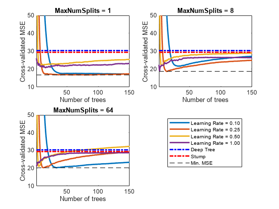
Each curve contains a minimum cross-validated MSE occurring at the optimal number of trees in the ensemble.
Identify the maximum number of splits, number of trees, and learning rate that yields the lowest MSE overall.
[minErr,minErrIdxLin] = min(error(:));
[idxNumTrees,idxMNS,idxLR] = ind2sub(size(error),minErrIdxLin);
fprintf('\nMin. MSE = %0.5f',minErr)
Min. MSE = 16.77593
fprintf('\nOptimal Parameter Values:\nNum. Trees = %d',idxNumTrees);Optimal Parameter Values: Num. Trees = 78
fprintf('\nMaxNumSplits = %d\nLearning Rate = %0.2f\n',...
    maxNumSplits(idxMNS),learnRate(idxLR))
MaxNumSplits = 1
Learning Rate = 0.25
Create a predictive ensemble based on the optimal hyperparameters and the entire training set.
tFinal = templateTree('MaxNumSplits',maxNumSplits(idxMNS),'Surrogate','on');
MdlFinal = fitrensemble(Tbl,'MPG','NumLearningCycles',idxNumTrees, ...
    'Learners',tFinal,'LearnRate',learnRate(idxLR))
MdlFinal =
  RegressionEnsemble
           PredictorNames: {'Cylinders'  'Displacement'  'Horsepower'  'Weight'}
             ResponseName: 'MPG'
    CategoricalPredictors: []
        ResponseTransform: 'none'
          NumObservations: 94
               NumTrained: 78
                   Method: 'LSBoost'
             LearnerNames: {'Tree'}
     ReasonForTermination: 'Terminated normally after completing the requested number of training cycles.'
                  FitInfo: [78×1 double]
       FitInfoDescription: {2×1 cell}
           Regularization: []


  Properties, Methods
MdlFinal is a RegressionEnsemble. To predict the fuel economy of a car given its number of cylinders, volume displaced by the cylinders, horsepower, and weight, you can pass the predictor data and MdlFinal to predict.
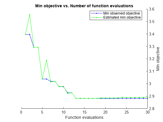
Instead of searching optimal values manually by using the cross-validation option ('KFold') and the kfoldLoss function, you can use the 'OptimizeHyperparameters' name-value pair argument. When you specify 'OptimizeHyperparameters', the software finds optimal parameters automatically using Bayesian optimization. The optimal values obtained by using 'OptimizeHyperparameters' can be different from those obtained using manual search.
t = templateTree('Surrogate','on');
mdl = fitrensemble(Tbl,'MPG','Learners',t, ...
    'OptimizeHyperparameters',{'NumLearningCycles','LearnRate','MaxNumSplits'})
|====================================================================================================================|
| Iter | Eval   | Objective:  | Objective   | BestSoFar   | BestSoFar   | NumLearningC-|    LearnRate | MaxNumSplits |
|      | result | log(1+loss) | runtime     | (observed)  | (estim.)    | ycles        |              |              |
|====================================================================================================================|
|    1 | Best   |      3.3955 |     0.27764 |      3.3955 |      3.3955 |           26 |     0.072054 |            3 |
|    2 | Accept |      6.0976 |     0.38981 |      3.3955 |      3.5549 |          170 |    0.0010295 |           70 |
|    3 | Best   |      3.2914 |     0.49048 |      3.2914 |      3.2917 |          273 |      0.61026 |            6 |
|    4 | Accept |      6.1839 |     0.11118 |      3.2914 |      3.2915 |           80 |    0.0016871 |            1 |
|    5 | Best   |      3.0379 |     0.08038 |      3.0379 |      3.0384 |           18 |      0.21288 |           37 |
|    6 | Accept |       3.169 |      0.4818 |      3.0379 |      3.0397 |          369 |      0.17992 |            4 |
|    7 | Accept |      3.0501 |    0.045081 |      3.0379 |      3.0402 |           10 |      0.28387 |           44 |
|    8 | Accept |      3.5336 |    0.047223 |      3.0379 |      3.1625 |           10 |      0.16084 |           99 |
|    9 | Best   |      2.9907 |    0.046076 |      2.9907 |      3.1233 |           12 |       0.3484 |            3 |
|   10 | Best   |      2.9378 |    0.043398 |      2.9378 |       2.968 |           11 |       0.3631 |            4 |
|   11 | Accept |      2.9629 |    0.030803 |      2.9378 |       2.943 |           10 |       0.2995 |            1 |
|   12 | Accept |      3.1123 |    0.029387 |      2.9378 |      2.9337 |           10 |      0.95361 |            1 |
|   13 | Best   |      2.9067 |    0.076107 |      2.9067 |      2.9493 |           71 |      0.30342 |            1 |
|   14 | Best   |      2.9016 |    0.083214 |      2.9016 |      2.9095 |           59 |      0.28365 |            1 |
|   15 | Accept |       5.891 |    0.031032 |      2.9016 |      2.9072 |           10 |     0.028505 |            1 |
|   16 | Accept |       6.318 |    0.032695 |      2.9016 |      2.9079 |           10 |    0.0064473 |            1 |
|   17 | Accept |      2.9406 |     0.40265 |      2.9016 |      2.9282 |          494 |       0.2463 |            1 |
|   18 | Accept |       3.101 |    0.032536 |      2.9016 |      2.9189 |           10 |      0.23598 |            1 |
|   19 | Accept |      3.3256 |      1.0379 |      2.9016 |      2.9085 |          500 |      0.33176 |           66 |
|   20 | Accept |      2.9474 |    0.032808 |      2.9016 |      2.9062 |           10 |      0.51189 |            1 |
|====================================================================================================================|
| Iter | Eval   | Objective:  | Objective   | BestSoFar   | BestSoFar   | NumLearningC-|    LearnRate | MaxNumSplits |
|      | result | log(1+loss) | runtime     | (observed)  | (estim.)    | ycles        |              |              |
|====================================================================================================================|
|   21 | Accept |      2.9906 |    0.040708 |      2.9016 |      2.9105 |           10 |      0.26521 |            7 |
|   22 | Accept |      2.9384 |    0.032004 |      2.9016 |      2.9066 |           10 |      0.41211 |            1 |
|   23 | Accept |      3.2353 |    0.043367 |      2.9016 |      2.9034 |           10 |      0.76556 |           98 |
|   24 | Accept |      3.0165 |    0.029857 |      2.9016 |      2.9021 |           10 |       0.6993 |            1 |
|   25 | Accept |      2.9599 |    0.083848 |      2.9016 |      2.9214 |           72 |      0.25746 |            2 |
|   26 | Best   |      2.8927 |    0.031856 |      2.8927 |       2.912 |           10 |      0.37133 |            1 |
|   27 | Best   |      2.8783 |    0.030043 |      2.8783 |      2.9011 |           10 |      0.36962 |            1 |
|   28 | Accept |      2.8895 |    0.030452 |      2.8783 |      2.8978 |           10 |      0.36592 |            1 |
|   29 | Accept |      2.8908 |    0.030437 |      2.8783 |       2.896 |           10 |      0.36275 |            1 |
|   30 | Accept |      6.1839 |    0.063397 |      2.8783 |       2.896 |           10 |     0.013418 |            1 |

__________________________________________________________
Optimization completed.
MaxObjectiveEvaluations of 30 reached.
Total function evaluations: 30
Total elapsed time: 12.208 seconds
Total objective function evaluation time: 4.2182

Best observed feasible point:
    NumLearningCycles    LearnRate    MaxNumSplits
    _________________    _________    ____________

           10             0.36962          1

Observed objective function value = 2.8783
Estimated objective function value = 2.896
Function evaluation time = 0.030043

Best estimated feasible point (according to models):
    NumLearningCycles    LearnRate    MaxNumSplits
    _________________    _________    ____________

           10             0.36962          1

Estimated objective function value = 2.896
Estimated function evaluation time = 0.031984
mdl =
  RegressionEnsemble
                       PredictorNames: {'Cylinders'  'Displacement'  'Horsepower'  'Weight'}
                         ResponseName: 'MPG'
                CategoricalPredictors: []
                    ResponseTransform: 'none'
                      NumObservations: 94
    HyperparameterOptimizationResults: [1×1 classreg.learning.paramoptim.SupervisedLearningBayesianOptimization]
                           NumTrained: 10
                               Method: 'LSBoost'
                         LearnerNames: {'Tree'}
                 ReasonForTermination: 'Terminated normally after completing the requested number of training cycles.'
                              FitInfo: [10×1 double]
                   FitInfoDescription: {2×1 cell}
                       Regularization: []


  Properties, Methods
Load the carsmall data set. Consider a model that predicts the mean fuel economy of a car given its acceleration, number of cylinders, engine displacement, horsepower, manufacturer, model year, and weight. Consider Cylinders, Mfg, and Model_Year as categorical variables.
load carsmall
Cylinders = categorical(Cylinders);
Mfg = categorical(cellstr(Mfg));
Model_Year = categorical(Model_Year);
X = table(Acceleration,Cylinders,Displacement,Horsepower,Mfg,...
    Model_Year,Weight,MPG);
Display the number of categories represented in the categorical variables.
numCylinders = numel(categories(Cylinders))
numCylinders =
3
numMfg = numel(categories(Mfg))
numMfg =
28
numModelYear = numel(categories(Model_Year))
numModelYear =
3
Because there are 3 categories only in Cylinders and Model_Year, the standard CART, predictor-splitting algorithm prefers splitting a continuous predictor over these two variables.
Train a random forest of 500 regression trees using the entire data set. To grow unbiased trees, specify usage of the curvature test for splitting predictors. Because there are missing values in the data, specify usage of surrogate splits. To reproduce random predictor selections, set the seed of the random number generator by using rng and specify 'Reproducible',true.
rng('default'); % For reproducibility
t = templateTree('PredictorSelection','curvature','Surrogate','on', ...
    'Reproducible',true); % For reproducibility of random predictor selections
Mdl = fitrensemble(X,'MPG','Method','bag','NumLearningCycles',500, ...
    'Learners',t);
Estimate predictor importance measures by permuting out-of-bag observations. Perform calculations in parallel.
options = statset('UseParallel',true);
imp = oobPermutedPredictorImportance(Mdl,'Options',options);
Starting parallel pool (parpool) using the 'Processes' profile ...
18-Aug-2025 13:34:21: Job Running. Waiting for parallel pool workers to connect ...
Connected to parallel pool with 6 workers.
Compare the estimates using a bar graph.
figure;
bar(imp);
title('Out-of-Bag Permuted Predictor Importance Estimates');
ylabel('Estimates');
xlabel('Predictors');
h = gca;
h.XTickLabel = Mdl.PredictorNames;
h.XTickLabelRotation = 45;
h.TickLabelInterpreter = 'none';
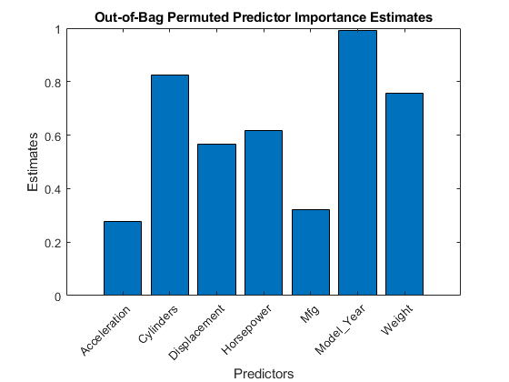
In this case, Model_Year is the most important predictor, followed by Cylinders. Compare these results to the results in Estimate Importance of Predictors.
Create an ensemble template for use in fitcecoc.
Load the arrhythmia data set.
load arrhythmia
tabulate(categorical(Y));
Value Count Percent
1 245 54.20%
2 44 9.73%
3 15 3.32%
4 15 3.32%
5 13 2.88%
6 25 5.53%
7 3 0.66%
8 2 0.44%
9 9 1.99%
10 50 11.06%
14 4 0.88%
15 5 1.11%
16 22 4.87%
rng(1); % For reproducibilitySome classes have small relative frequencies in the data.
Create a template for a AdaBoostM1 ensemble of classification trees, and specify to use 100 learners and a shrinkage of 0.1. By default, boosting grows stumps (i.e., one node having a set of leaves). Since there are classes with small frequencies, the trees must be leafy enough to be sensitive to the minority classes. Specify the minimum number of leaf node observations to 3.
tTree = templateTree('MinLeafSize',20);
t = templateEnsemble('AdaBoostM1',100,tTree,'LearnRate',0.1);
All properties of the template objects are empty except for Method and Type, and the corresponding properties of the name-value pair argument values in the function calls. When you pass t to the training function, the software fills in the empty properties with their respective default values.
Specify t as a binary learner for an ECOC multiclass model. Train using the default one-versus-one coding design.
Mdl = fitcecoc(X,Y,'Learners',t);Mdlis aClassificationECOCmulticlass model.Mdl.BinaryLearnersis a 78-by-1 cell array ofCompactClassificationEnsemblemodels.Mdl.BinaryLearners{j}.Trainedis a 100-by-1 cell array ofCompactClassificationTreemodels, forj= 1,...,78.
You can verify that one of the binary learners contains a weak learner that isn't a stump by using view.
view(Mdl.BinaryLearners{1}.Trained{1},'Mode','graph')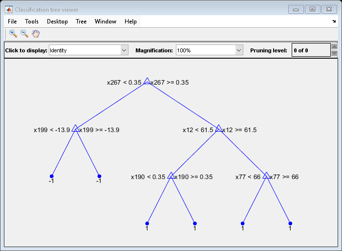
Display the in-sample (resubstitution) misclassification error.
L = resubLoss(Mdl,'LossFun','classiferror')
L =
0.0819
Name-Value Arguments
Output Arguments
Algorithms
To accommodate
MaxNumSplits, the software splits all nodes in the current layer, and then counts the number of branch nodes. A layer is the set of nodes that are equidistant from the root node. If the number of branch nodes exceedsMaxNumSplits, then the software follows this procedure.Determine how many branch nodes in the current layer need to be unsplit so that there would be at most
MaxNumSplitsbranch nodes.Sort the branch nodes by their impurity gains.
Unsplit the desired number of least successful branches.
Return the decision tree grown so far.
This procedure aims at producing maximally balanced trees.
The software splits branch nodes layer by layer until at least one of these events occurs.
There are
MaxNumSplits+ 1 branch nodes.A proposed split causes the number of observations in at least one branch node to be fewer than
MinParentSize.A proposed split causes the number of observations in at least one leaf node to be fewer than
MinLeafSize.The algorithm cannot find a good split within a layer (i.e., the pruning criterion (see
PruneCriterion), does not improve for all proposed splits in a layer). A special case of this event is when all nodes are pure (i.e., all observations in the node have the same class).For values
'curvature'or'interaction-curvature'ofPredictorSelection, all tests yield p-values greater than 0.05.
MaxNumSplitsandMinLeafSizedo not affect splitting at their default values. Therefore, if you set'MaxNumSplits', then splitting might stop due to the value ofMinParentSizebeforeMaxNumSplitssplits occur.For details on selecting split predictors and node-splitting algorithms when growing decision trees, see Algorithms for classification trees and Algorithms for regression trees.
References
[1] Breiman, L., J. Friedman, R. Olshen, and C. Stone. Classification and Regression Trees. Boca Raton, FL: CRC Press, 1984.
[2] Coppersmith, D., S. J. Hong, and J. R. M. Hosking. “Partitioning Nominal Attributes in Decision Trees.” Data Mining and Knowledge Discovery, Vol. 3, 1999, pp. 197–217.
[3] Loh, W.Y. “Regression Trees with Unbiased Variable Selection and Interaction Detection.” Statistica Sinica, Vol. 12, 2002, pp. 361–386.
[4] Loh, W.Y. and Y.S. Shih. “Split Selection Methods for Classification Trees.” Statistica Sinica, Vol. 7, 1997, pp. 815–840.
Version History
Introduced in R2014a
See Also
ClassificationTree | RegressionTree | fitctree | fitcensemble | fitrensemble | fitcecoc | templateEnsemble