Out-of-Distribution Detection for LSTM Document Classifier

Since R2024a

This example uses:

This example shows how to detect out-of-distribution (OOD) data in an LSTM document classifier.

OOD data detection is the process of identifying inputs to a deep neural network that might yield unreliable predictions. OOD data refers to data that is different from the data used to train the model, for example, data collected in a different way, under different conditions, or for a different task than the data on which the model was originally trained.

You can classify data as in-distribution (ID) or OOD by assigning confidence scores to the predictions of a network. You can then choose how you treat OOD data. For example, you can choose to reject the prediction of a neural network if the network detects OOD data.

In this example, you train an LSTM classification model to predict the type of maintenance work done on traffic signals using text descriptions. You then construct a discriminator to classify the text descriptions as ID or OOD.

In this example, you train and use the LSTM network in five steps:

Import and preprocess the data.
Separate the ID and OOD data.
Convert the words to numeric sequences using a word encoding.
Create and train an LSTM network with a word embedding layer using the ID data.
Construct a distribution discriminator and compare distribution scores for ID and OOD data.

Import and Preprocess Data

This example uses a large data set that contains records of work completed by traffic signal technicians in the city of Austin, TX, United States [1]. This data set is a table containing approximately 36,000 reports with various attributes, including a plain text description in the JobDescription variable and a categorical label in the WorkNeeded variable.

Load the example data.

zipFile = matlab.internal.examples.downloadSupportFile("textanalytics","data/Traffic_Signal_Work_Orders.zip");
filepath = fileparts(zipFile);
dataFolder = fullfile(filepath,"Traffic_Signal_Work_Orders");
unzip(zipFile,dataFolder);
filename = "Traffic_Signal_Work_Orders.csv";
data = readtable(fullfile(dataFolder,filename),TextType="string", VariableNamingRule="preserve");
data.Properties.VariableNames = matlab.lang.makeValidName(data.Properties.VariableNames);
head(data)

     WorkOrderID       Status        AssetType        AssetID      LocationID               CreatedDate                       ModifiedDate                     SubmittedDate                       ClosedDate              FiscalYear        WorkType                                  WorkNeeded                                                           WorkTypeOther                                       WorkRequestedBy                                          JobDescription                                                                                              ProblemFound                                                                                                                                                                                 ActionTaken                                                                                                                        Follow_UpNeeded    ChildWorkOrder    ParentWorkOrder    IsFollow_Up      TMCIssueID      ServiceRequest_    DamageReport                             LocationName                             Latitude    Longitude               Location           
    ______________    ________    ________________    _______    ______________    ______________________________    ______________________________    ______________________________    ______________________________    __________    ________________    _______________________________________________________________    _____________________________________________________________________    _____________________________    _____________________________________________________________________________    ________________________________________________________________________________________________________________________________    __________________________________________________________________________________________________________________________________________________________________________________________________________________________________________________    _______________    ______________    _______________    ___________    ______________    _______________    ____________    ______________________________________________________________    ________    _________    ______________________________

    "WRK17-001685"    "Closed"    "School Flasher"      NaN      <missing>         "08/19/2017 08:55:00 PM +0000"    "09/14/2017 06:27:00 PM +0000"    "08/19/2017 09:00:00 PM +0000"    "09/14/2017 06:27:00 PM +0000"       2017       "Scheduled Work"    "Call-Back (Test Monitors and Cabinets)"                           <missing>                                                                "Austin Transportation Staff"    "HAVE AUSTIN ENERGY TIE IN NEW SOURCE DROP OVERHEAD @ CIMA SERENA WB FLASHER"    "N/A."                                                                                                                              "AUSTIN ENERGY TECHNICIANS DISPATCHED TO LOCATION. AE TECHS COULD NOT DO WORK BECAUSE OF LACK OF METER ON POLE/SOURCE. AE TECHS SAID TO CONTACT "WORK MANAGMENT NORTH" 5125057179 FOR FURTHER ACTION. INFORMATION WILL BE RELAYED TO SUPERVISOR. "        "False"          <missing>          <missing>        <missing>     <missing>          <missing>          <missing>      <missing>                                                           NaN          NaN       <missing>                     
    "WRK17-001865"    "Closed"    "Signal"              317      "LOC16-001550"    "08/24/2017 03:28:00 PM +0000"    "09/14/2017 06:42:00 PM +0000"    "08/24/2017 03:56:00 PM +0000"    "09/14/2017 06:42:00 PM +0000"       2017       "Scheduled Work"    "Installation - Other"                                             <missing>                                                                "Austin Transportation Staff"    <missing>                                                                        "bad cable for nb in the conduits"                                                                                                  "pulled in 20 conductor cable for nb signals and peds . installed a new 332 cabinet , respliced all signals and peds for 2 way project ."                                                                                                                 "False"          <missing>          <missing>        <missing>     <missing>          <missing>          <missing>      "5TH ST / TRINITY ST"                                               NaN          NaN       "POINT (-97.739677 30.266132)"
    "WRK17-001875"    "Closed"    "Signal"              319      "LOC16-001560"    "08/24/2017 03:45:00 PM +0000"    "09/14/2017 06:54:00 PM +0000"    "08/24/2017 04:03:00 PM +0000"    "09/14/2017 06:54:00 PM +0000"       2017       "Scheduled Work"    "Installation - Other"                                             <missing>                                                                "MMC"                            "install wb standard and splice in signals and peds"                             <missing>                                                                                                                           "install wb mast arm, remove street light pole, splice signal cables and peds"                                                                                                                                                                            "False"          <missing>          <missing>        <missing>     <missing>          <missing>          <missing>      "5TH ST / RED RIVER ST"                                             NaN          NaN       "POINT (-97.737488 30.265535)"
    "WRK17-001890"    "Closed"    "School Flasher"      NaN      <missing>         "08/24/2017 08:23:00 PM +0000"    "08/24/2017 08:31:00 PM +0000"    "08/24/2017 08:31:00 PM +0000"    "08/28/2017 03:08:00 PM +0000"       2017       "Trouble Call"      "OtherDay-Call (Deliver Timing sheets to intersections and PM)"    "SOMMERS ELEMENTARY - NOT FLASHING↵↵SR #17-00242843↵#17-00244051↵"    "Austin Transportation Staff"    "SOMMERS ELEMENTARY - NOT FLASHING↵SR #17-00242843, #17-00244051"               "NO PROBLEMS FOUND AT SCHOOL FLASHERS.  BOTH PEDESTRIAN FLASHERS NEED SCHEDULE."                                                    "BOTH SCHOOL CLOCKS CHECKED FOR TIME, DATE, SCHEDULE, FLASHERS OPERATION AND COMMUNICATION.↵BOTH PEDESTRIAN FLASHER CLOCKS CHECKED FOR TIME, DATE, SCHEDULE, OPERATION, AND COMM.↵TIME, DATE AND SCHEDULE UPDATED IN PEDESTRIAN FLASHER CLOCKS."         "False"          <missing>          <missing>        <missing>     <missing>          <missing>          <missing>      <missing>                                                           NaN          NaN       <missing>                     
    "WRK17-003185"    "Closed"    "Signal"               25      "LOC16-000120"    "10/09/2017 07:46:00 PM +0000"    "01/23/2023 04:47:00 PM +0000"    "10/09/2017 07:49:00 PM +0000"    "10/10/2017 04:45:00 PM +0000"       2018       "Scheduled Work"    "Installation - Camera"                                            <missing>                                                                "MMC"                            "replace the avidia cctv with a pelco repaired unit"                             <missing>                                                                                                                           "replaced the avidia cctv with a repaired pelco task # 2423015000"                                                                                                                                                                                        "False"          <missing>          <missing>        <missing>     <missing>          <missing>          <missing>      "MARTIN LUTHER KING JR BLVD / CONGRESS AVE (MLK/Capitol Mall)"      NaN          NaN       "POINT (-97.738106 30.280687)"
    "WRK17-003430"    "Closed"    "Signal"              185      "LOC16-000915"    "10/18/2017 08:43:00 PM +0000"    "10/26/2017 07:30:00 PM +0000"    "10/18/2017 08:49:00 PM +0000"    "10/26/2017 07:30:00 PM +0000"       2018       "Trouble Call"      "Visibility Issue"                                                 <missing>                                                                "MMC"                            "Tree limbs blocking WB signal direction."                                       "Tree limbs blocking WB signal direction."                                                                                          "Cut limbs blocking WB signal direction to make visible for ongoing traffic."                                                                                                                                                                             "True"           <missing>          <missing>        <missing>     "TMC17-006530"     "17-00311041"      <missing>      "LAMAR BLVD / PANTHER TRL"                                          NaN          NaN       "POINT (-97.789284 30.23867)" 
    "WRK17-001895"    "Closed"    "Signal"              NaN      <missing>         "08/24/2017 08:32:00 PM +0000"    "08/24/2017 08:40:00 PM +0000"    "08/24/2017 08:40:00 PM +0000"    "08/28/2017 03:06:00 PM +0000"       2017       "Trouble Call"      "OtherDay-Call (Deliver Timing sheets to intersections and PM)"    "DOSS/MURCHISON COMBO WB NOT FLASHING"                                   "Austin Transportation Staff"    "DOSS/MURCHISON COMBO WB NOT FLASHING"                                           "WB FLASHER ON GREYSTONE  DOES NOT HAVE COMMUNICATION. CLOCK HAD NO SCHEDULE.  EB FLASHER ON N HILLS DR. HAS LIMBS OBSTRUCTION."    "DATE, TIME, SCHEDULE, AND FLASHER OPERATION CHECKED FOR ALL CLCOKS. WB CLOCK ON GREYSTONE PROGRAMMED WITH 2017/2018 SCHEDULE. LIMBS REMOVED FROM EB FLASHER ON N HILLS DR."                                                                              "False"          <missing>          <missing>        <missing>     <missing>          <missing>          <missing>      <missing>                                                           NaN          NaN       <missing>                     
    "WRK17-002010"    "Closed"    "Signal"              779      "LOC16-003835"    "08/29/2017 07:58:00 PM +0000"    "09/14/2017 07:04:00 PM +0000"    "08/30/2017 11:02:00 AM +0000"    "09/14/2017 07:04:00 PM +0000"       2017       "Trouble Call"      "Detection Failure"                                                <missing>                                                                "MMC"                            "fisheye camera turned"                                                          "gridsmart camera out of alignment"                                                                                                 "with assistance from the TMC - realigned camera and tightened"                                                                                                                                                                                           "False"          <missing>          <missing>        <missing>     <missing>          <missing>          <missing>      "MC KINNEY FALLS PKWY / WILLIAM CANNON DR"                          NaN          NaN       "POINT (-97.72583 30.163218)"

The goal of this example is to classify maintenance visits by the label in the WorkNeeded column. To divide the data into classes, convert these labels to categorical.

data.WorkNeeded = categorical(data.WorkNeeded);

Split the data into two data sets, commonData and rareData, depending on whether the WorkNeeded category occurs more or less often than 500 times. To find how many instances of each category are present, use the countcats function.

workNeededCategories = categories(data.WorkNeeded);
categoryFrequencies = countcats(data.WorkNeeded);

commonCategories = workNeededCategories(categoryFrequencies>500);
rareCategories = workNeededCategories(categoryFrequencies<=500);

commonData = data(ismember(data.WorkNeeded,commonCategories),:);
rareData = data(ismember(data.WorkNeeded,rareCategories),:);

Remove miscellaneous categories from the common data and add them to the rare data.

otherCategories = commonCategories(contains(commonCategories,"Other"));
commonData = commonData(~ismember(commonData.WorkNeeded,otherCategories),:);
rareData = [rareData; data(ismember(data.WorkNeeded,otherCategories),:)];

Remove now unused categories.

commonData.WorkNeeded = removecats(commonData.WorkNeeded);
rareData.WorkNeeded = removecats(rareData.WorkNeeded);

Separate ID and OOD Data

In this example, you train a document classifier on the JobDescription fields of the reports that result in the most common WorkNeeded categories. This data comprises the ID data.

dataID = commonData;

To determine whether a given JobDescription is similar to the training data, you then construct a distribution discriminator. Set aside the data from the rare categories as OOD data.

dataOOD = rareData;

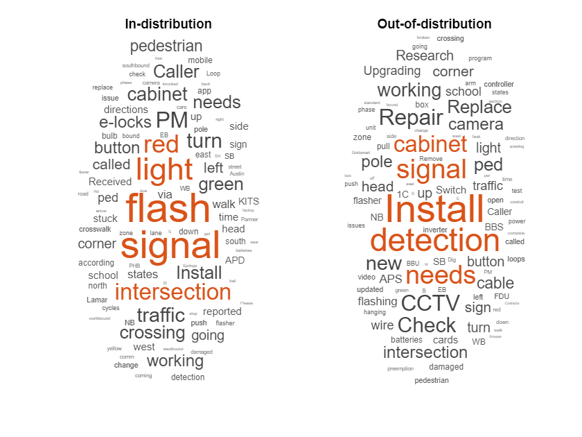
Compare the JobDescription fields of both ID and OOD data using word clouds.

figure
tiledlayout("horizontal")
nexttile
wordcloud(dataID.JobDescription);
title("In-distribution")
nexttile
wordcloud(dataOOD.JobDescription);
title("Out-of-distribution")

Prepare Data for Training

Next, partition the ID data into sets for training, validation, and testing. Partition the data into a training set containing 80% of the ID data, a validation set containing 10% of the ID data, and a test set containing the remaining 10% of the ID data. To partition the data, use the trainingPartitions function, attached to this example as a supporting file. To access this file, open the example as a live script.

numReports = size(dataID,1);
[idxTrain,idxValidation,idxTest] = trainingPartitions(numReports,[0.8 0.1 0.1]);

dataTrain = dataID(idxTrain,:);
dataValidation = dataID(idxValidation,:);
dataTest = dataID(idxTest,:);

Extract the text data and labels from the partitioned tables and the OOD data.

textDataTrain = dataTrain.JobDescription;
textDataValidation = dataValidation.JobDescription;
textDataTest = dataTest.JobDescription;
textDataOOD = dataOOD.JobDescription;

YTrain = dataTrain.WorkNeeded;
YValidation = dataValidation.WorkNeeded;
YTest = dataTest.WorkNeeded;
YOOD = dataOOD.WorkNeeded;

Preprocess Text Data

Create a function that tokenizes and preprocesses the text data. The function performs these steps:

Tokenize the text using tokenizedDocument.
Add token details using addPartOfSpeechDetails.
Convert the text to lowercase using lower.
Remove words shorter than two letters using removeShortWords.
Remove words longer than 15 letters using removeLongWords.
Remove words like "a," "to," and "the" using removeStopWords.
Erase the punctuation using erasePunctuation.
Remove now empty documents using removeEmptyDocuments. The function also returns the indices of the documents that it removed.

function [preprocessedText,idx] = preprocessText(textData)
preprocessedText = tokenizedDocument(textData);
preprocessedText = addPartOfSpeechDetails(preprocessedText);
preprocessedText = lower(preprocessedText);
preprocessedText = normalizeWords(preprocessedText,Style="lemma");
preprocessedText = removeShortWords(preprocessedText,2);
preprocessedText = removeLongWords(preprocessedText,15);
preprocessedText = removeStopWords(preprocessedText,IgnoreCase=false);
preprocessedText = erasePunctuation(preprocessedText);
[preprocessedText,idx] = removeEmptyDocuments(preprocessedText);
end

Preprocess the training, validation, testing, and OOD data using the preprocessText function. Remove the data rows now containing empty documents in the WorkNeeded column.

[documentsTrain,idxTrain] = preprocessText(textDataTrain);
[documentsValidation,idxValidation] = preprocessText(textDataValidation);
[documentsTest,idxTest] = preprocessText(textDataTest);
[documentsOOD,idxOOD] = preprocessText(textDataOOD);

YTrain(idxTrain) = [];
YValidation(idxValidation) = [];
YTest(idxTest) = [];
YOOD(idxOOD) = [];

View the first few preprocessed training documents.

documentsTrain(1:5)

ans = 
  5×1 tokenizedDocument:

    7 tokens: martin luther king jr red river flash
    2 tokens: check comm
    5 tokens: bolm airport shady airport intersection
    6 tokens: 834 tannehill martin luther king blvd
    7 tokens: face wrong side street due high wind

Convert Document to Sequences

To input the documents into an LSTM network, use a word encoding to convert the documents into sequences of numeric indices.

To create a word encoding, use the wordEncoding function.

enc = wordEncoding(documentsTrain);

The next conversion step is to pad and truncate documents so that they are all the same length. The trainingOptions (Deep Learning Toolbox) function provides options to pad and truncate input sequences automatically. However, these options are not well suited for sequences of word vectors. Instead, pad and truncate the sequences manually. If you left-pad and truncate the sequences of word vectors, then the training might improve.

To pad and truncate the documents, first choose a target length, and then truncate documents that are longer than it and left-pad documents that are shorter than it. For best results, use target lengths that are short but not so short that you must discard large amounts of data. To find a suitable target length, view a histogram of the training document lengths.

documentLengths = doclength(documentsTrain);
figure
histogram(documentLengths)
xlim([0 20])
title("Document Lengths")
xlabel("Length")
ylabel("Number of Documents")

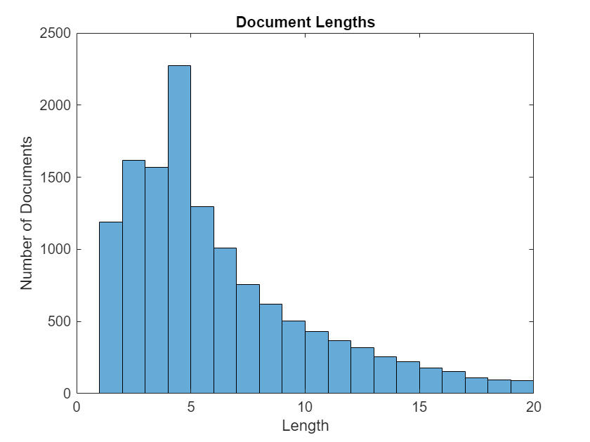
Convert the documents to sequences of numeric indices using the doc2sequence function. To truncate or left-pad the sequences to have a length of 10, set the Length option to 10.

sequenceLength = 10;
XTrain = doc2sequence(enc,documentsTrain,Length=sequenceLength);
XValidation = doc2sequence(enc,documentsValidation,Length=sequenceLength);
XTest = doc2sequence(enc,documentsTest,Length=sequenceLength);

Create and Train LSTM Network

Define the LSTM network architecture. To input sequence data into the network, include a sequence input layer and set the input size to 1. Next, include a word embedding layer of dimension 50 and the same number of words as the word encoding. Next, include an LSTM layer and set the number of hidden units to 80. To use the LSTM layer for a sequence-to-label classification problem, set the output mode to "last". Finally, add a fully connected layer with the same size as the number of classes, as well as a softmax layer.

inputSize = 1;
embeddingDimension = 50;
numHiddenUnits = 80;

numWords = enc.NumWords;
classNames = categories(YTrain);
numClasses = numel(classNames);

layers = [ ...
    sequenceInputLayer(inputSize)
    wordEmbeddingLayer(embeddingDimension,numWords)
    lstmLayer(numHiddenUnits,OutputMode="last")
    fullyConnectedLayer(numClasses)
    softmaxLayer]

layers = 
  5×1 Layer array with layers:

     1   ''   Sequence Input         Sequence input with 1 dimensions
     2   ''   Word Embedding Layer   Word embedding layer with 50 dimensions and 5677 unique words
     3   ''   LSTM                   LSTM with 80 hidden units
     4   ''   Fully Connected        11 fully connected layer
     5   ''   Softmax                softmax

Specify Training Options

Specify the training options:

Train using the Adam solver.
Shuffle the data every epoch.
Monitor the training progress by setting the Plots option to "training-progress".
Monitor the accuracy in addition to the loss during training by setting the Metrics option to "accuracy".
Specify the validation data using the ValidationData option.
Set the ValidationFrequency to 10.
Set the ValidationPatience to 5.
Suppress verbose output by setting the Verbose option to false.
Specify that the input data has the format "CTB" (channel, time, batch).

options = trainingOptions("adam", ...
    GradientThreshold=2, ...
    MaxEpochs=20, ...
    Shuffle="every-epoch", ...
    ValidationData={XValidation,YValidation}, ...
    ValidationFrequency=10, ...
    ValidationPatience=5, ...
    Metrics="accuracy", ...
    Plots="training-progress", ...
    Verbose=false, ...
    InputDataFormats="CTB");

Train the LSTM network using the trainnet (Deep Learning Toolbox) function.

net = trainnet(XTrain,YTrain,layers,"crossentropy",options);

Test Neural Network

Make predictions using the test data.

scores = minibatchpredict(net,XTest,InputDataFormats="CTB");
YPred = scores2label(scores,classNames);

Calculate the accuracy.

accuracy = nnz(YTest==YPred)/numel(YPred)

accuracy = 
0.8152

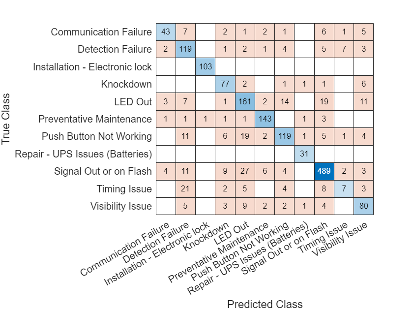
To illustrate the predictions of the model, plot a confusion chart using the confusionchart (Deep Learning Toolbox) function.

figure
confusionchart(YTest,YPred)

Detect OOD Data

Convert the OOD documents to sequences of numeric indices using the doc2sequence function. Convert the ID and OOD data to dlarray (Deep Learning Toolbox).

XOOD = doc2sequence(enc,documentsOOD,Length=sequenceLength);
XOOD = dlarray(cat(3,XOOD{:}),"CTB");
XID = dlarray(cat(3,XTrain{:}),"CTB");

You can assign confidence scores to network predictions by computing a distribution confidence score for each observation. ID data usually has a higher confidence score than OOD data. You can then apply a threshold to the scores to determine whether an input is ID or OOD.

Create a discriminator that separates ID and OOD data by using the networkDistributionDiscriminator (Deep Learning Toolbox) function. The function returns a discriminator containing a threshold for separating data into ID and OOD using their distribution scores. To specify the algorithm used by networkDistributionDiscriminator, set the method input argument to BaselineDistributionDiscriminator (Deep Learning Toolbox), ODINDistributionDiscriminator (Deep Learning Toolbox), EnergyDistributionDiscriminator (Deep Learning Toolbox), or HBOSDistributionDiscriminator (Deep Learning Toolbox).

Use Baseline Distribution Discriminator

Create a distribution discriminator using the baseline OOD discrimination algorithm. The baseline method computes distribution confidence scores based on softmax scores. The method directly compares softmax scores associated with different predictions. For more information, see Distribution Confidence Scores (Deep Learning Toolbox).

discriminatorBaseline = networkDistributionDiscriminator(net,XID,XOOD,"baseline");

Pass the discriminator object to the isInNetworkDistribution (Deep Learning Toolbox) function along with the ID or OOD data. To assess the performance of the discriminator, calculate the true positive rate (TPR) and false positive rate (FPR).

tfOODBaseline = isInNetworkDistribution(discriminatorBaseline,XOOD);
tfIDBaseline = isInNetworkDistribution(discriminatorBaseline,XID);
TPRBaseline = nnz(tfIDBaseline)/numel(tfIDBaseline)

TPRBaseline = 
0.5470

FPRBaseline = nnz(tfOODBaseline)/numel(tfOODBaseline)

FPRBaseline = 
0.1441

To calculate the distribution scores and distribution threshold of ID and OOD data according to the discriminator, pass the discriminator object to the distributionScores (Deep Learning Toolbox) function. Plot a histogram of the distribution scores using the plotDistributionScores function, defined at the end of this example.

scoresIDBaseline = distributionScores(discriminatorBaseline,XID);
scoresOODBaseline = distributionScores(discriminatorBaseline,XOOD);
figure
plotDistributionScores(discriminatorBaseline,scoresIDBaseline,scoresOODBaseline)

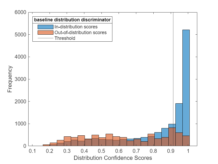
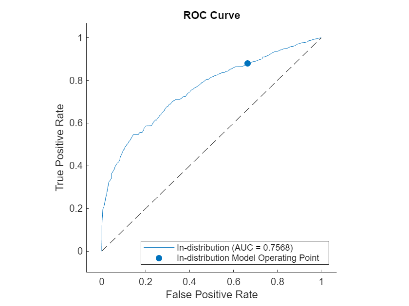
Find the receiver operating characteristic (ROC) curves for the ID and OOD data sets using the discriminator and the distribution scores. Use the rocmetrics function to compute the ROC metrics, including the area under the ROC curve (AUC). A discriminator that is able to separate ID and OOD data achieves an AUC value close to 1.

labels = [
    repelem("In-distribution",numel(scoresIDBaseline)), ...
    repelem("Out-of-distribution",numel(scoresOODBaseline))];
scoresBaseline = [scoresIDBaseline',scoresOODBaseline'];
rocObjBaseline = rocmetrics(labels,scoresBaseline,"In-distribution");

Plot the ROC curves. The ROC curves show that the discriminator can distinguish OOD data from the ID data.

figure
plot(rocObjBaseline)

Use Energy Distribution Discriminator

Create a distribution discriminator using the energy distribution discrimination algorithm. The energy method computes distribution confidence scores based on softmax scores. For more information, see Distribution Confidence Scores (Deep Learning Toolbox).

Set the Temperature name-value argument to 1.

discriminatorEnergy = networkDistributionDiscriminator(net,XID,XOOD,"energy",Temperature=1);

Calculate the true and false positive rates. Plot the distribution scores. Plot the ROC curve.

tfOODEnergy = isInNetworkDistribution(discriminatorEnergy,XOOD);
tfIDEnergy = isInNetworkDistribution(discriminatorEnergy,XID);
TPREnergy = nnz(tfIDEnergy)/numel(tfIDEnergy)

TPREnergy = 
0.7173

FPREnergy = nnz(tfOODEnergy)/numel(tfOODEnergy)

FPREnergy = 
0.3188

scoresIDEnergy = distributionScores(discriminatorEnergy,XID);
scoresOODEnergy = distributionScores(discriminatorEnergy,XOOD);
figure
plotDistributionScores(discriminatorEnergy,scoresIDEnergy,scoresOODEnergy)

scoresEnergy = [scoresIDEnergy',scoresOODEnergy'];
rocObjEnergy = rocmetrics(labels,scoresEnergy,"In-distribution");