Out-of-Distribution Data Discriminator for YOLO v4 Object Detector

Prepare Training Data

This example uses a small vehicle data set that contains 295 images. Many of these images come from the Caltech Cars 1999 and 2001 data sets, created by Pietro Perona and used with permission. Each image contains one or two labeled instances of a vehicle. A small data set is useful for exploring the YOLO v4 training procedure, but in practice, more labeled images are needed to train a robust detector.

Unzip the vehicle images and load the vehicle ground truth data.

unzip vehicleDatasetImages.zip
data = load('vehicleDatasetGroundTruth.mat');
vehicleDataset = data.vehicleDataset;

Add the full path to the local vehicle data folder.

vehicleDataset.imageFilename = fullfile(pwd,vehicleDataset.imageFilename);

Split the data set into training and validation sets. Use 60% of the data for training and 40% for validation.

rng("default");
shuffledIndices = randperm(height(vehicleDataset));
idx = floor(0.6 * length(shuffledIndices));
trainingDataTbl = vehicleDataset(shuffledIndices(1:idx),:);
validationDataTbl = vehicleDataset(shuffledIndices(idx+1:end),:);

Use imageDatastore and boxLabelDatastore (Computer Vision Toolbox) to create datastores for loading the image and label data during training and validation.

imdsTrain = imageDatastore(trainingDataTbl.imageFilename);
bldsTrain = boxLabelDatastore(trainingDataTbl(:,"vehicle"));

imdsValidation = imageDatastore(validationDataTbl.imageFilename);
bldsValidation  = boxLabelDatastore(validationDataTbl(:,"vehicle"));

Combine the image and box label datastores.

dsTrain = combine(imdsTrain,bldsTrain);
dsValidation  = combine(imdsValidation,bldsValidation);

numObservationsTrain =  numel(imdsTrain.Files);
numObservationsValidation = numel(imdsValidation.Files);

Specify the input size to use for resizing the images and the bounding boxes. For the pretrained YOLO v4 detector, the underlying base networks require the size of the training images to be a multiple of 32.

inputSize = [224 224 3];

Estimate Anchor Boxes

Use the estimateAnchorBoxes (Computer Vision Toolbox) function to estimate anchor boxes based on the size of objects in the training data. To account for the resizing of the images prior to training, resize the training data for estimating anchor boxes. Use the transform function to preprocess the training data, then define the number of anchor boxes and estimate the anchor boxes. Resize the training data to the input size of the network by using the preprocessData helper function.

trainingDataForEstimation = transform(dsTrain,@(data)preprocessData(data,inputSize));

numAnchors = 6;
[anchors,meanIoU] = estimateAnchorBoxes(trainingDataForEstimation,numAnchors);

area = anchors(:,1).*anchors(:,2);
[~,idx] = sort(area,"descend");

anchors = anchors(idx,:);
anchorBoxes = {anchors(1:3,:);anchors(4:6,:)};

For more information about choosing anchor boxes, see Estimate Anchor Boxes From Training Data (Computer Vision Toolbox) and Anchor Boxes for Object Detection (Computer Vision Toolbox).

Configure and Train YOLO v4 Network

This example uses a YOLO v4 network pretrained on the COCO data set. In this example, you fine-tune the detector for detecting vehicles in an image. For more information on the fine-tuning and the vehicle data set used for the fine-tuning, see trainYOLOv4ObjectDetector (Computer Vision Toolbox).

Specify the class names and configure the pretrained YOLO v4 deep learning network for the new data set by using the yolov4ObjectDetector (Computer Vision Toolbox) function.

classes = "vehicle";
detector = yolov4ObjectDetector("tiny-yolov4-coco",classes,anchorBoxes,InputSize=inputSize);

Specify the training options and retrain the pretrained YOLO v4 network on the new data set by using the trainYOLOv4ObjectDetector function.

options = trainingOptions("sgdm", ...
    InitialLearnRate=0.001, ...
    MiniBatchSize=16, ...
    MaxEpochs=50, ...
    ValidationData=dsValidation, ...
    BatchNormalizationStatistics="moving", ...
    ResetInputNormalization=false, ...
    VerboseFrequency=30);

To save time, set the doTraining flag to false and load a pretrained network. If you want to train the detector, set the doTraining value to true.

doTraining = false;
if doTraining
    trainedDetector = trainYOLOv4ObjectDetector(dsTrain,detector,options);
else    
    filename = matlab.internal.examples.downloadSupportFile("nnet","data/trainedYolov4VehicleDetectionNetwork.mat");
    load(filename);
end

Examine the underlying backbone network for the YOLO v4 detector. For more information, see Getting Started with YOLO v4 (Computer Vision Toolbox).

net = trainedDetector.Network

net = 
  dlnetwork with properties:

         Layers: [74×1 nnet.cnn.layer.Layer]
    Connections: [80×2 table]
     Learnables: [80×3 table]
          State: [38×3 table]
     InputNames: {'input_1'}
    OutputNames: {'convOut1'  'convOut2'}
    Initialized: 1

  View summary with summary.

Detect Vehicles in Image

Load a sample image.

reset(dsTrain)
imgIdx = 1;
img = read(dsTrain);
img = img{imgIdx};

Normalize and resize the image.

img = im2single(img);
img = imresize(img,inputSize(1:2));

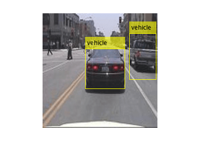
Detect vehicles and find the bounding boxes in the sample image.

detectorThr = 0.05;
[bboxes,~,labels] = detect(trainedDetector,img,Threshold=detectorThr);
detectedImage = insertObjectAnnotation(img,"Rectangle",bboxes,labels);

Display the image and bounding boxes.

figure
imshow(detectedImage)

Test Object Detector on OOD Data

The network can detect objects in images like those on which it was trained. Test how the network performs on data that you did not use during training.

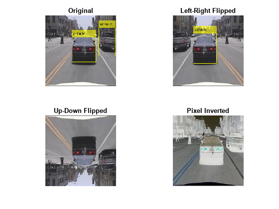
Augment the image to generate images different to those on which the network was trained. Use three types of image augmentation to generate the images:

imgLRFlip = fliplr(img);
imgUDFlip = flipud(img);
imgInvert = 1-img;

Use the fine-tuned YOLO v4 object detector to detect vehicles in the three augmented images.

[bboxesLRFlip,~,labelsLRFlip] = detect(trainedDetector,imgLRFlip,Threshold=detectorThr);
detectedLRFlip = insertObjectAnnotation(imgLRFlip,"Rectangle",bboxesLRFlip,labelsLRFlip);

[bboxesUDFlip,~,labelsUDFlip] = detect(trainedDetector,imgUDFlip,Threshold=detectorThr);
detectedUDFlip = insertObjectAnnotation(imgUDFlip,"Rectangle",bboxesUDFlip,labelsUDFlip);

[bboxesInvert,~,labelsInvert] = detect(trainedDetector,imgInvert,Threshold=detectorThr);
detectedInvert = insertObjectAnnotation(imgInvert,"Rectangle",bboxesInvert,labelsInvert);

Display the results for the original image and the augmented images using the helper function plotAugmentedImages, found at the end of this example. The network is unable to detect the car in the up-down flipped and the inverted images.

figure
plotAugmentedImages( ...
    detectedImage,"Original", ...
    detectedLRFlip,"Left-Right Flipped", ...
    detectedUDFlip,"Up-Down Flipped", ...
    detectedInvert,"Pixel Inverted")

When deploying models to safety-critical environments, it is important to have a method of assigning confidence to the network predictions. It is also important to have a method of classifying the image as outside of the distribution of data that the model has been trained on.

Create OOD Data Discriminator

You can assign confidence to network predictions by computing a distribution confidence score for each observation. ID data usually has a higher confidence score than OOD data [1]. You can then apply a threshold to the scores to determine whether an input is ID or OOD. The discriminator acts as an additional output of the trained network which classifies an observation as ID or OOD.

You can use the networkDistributionDiscriminator function to create a discriminator to separate data into ID and OOD. The function returns a discriminator containing a threshold for separating data into ID and OOD using their distribution scores.

To create a discriminator for a network with multiple outputs, you must have a set of ID data. The ID data must also be a dlarray object or a minibatchqueue object that returns a dlarray. In this example, you use the training data to create a data discriminator. Use the helper function convertToDlarray, found at the end of this example, to convert the data to a dlarray object. The helper function normalizes the data and resizes it to the input size the network expects. The function then returns a dlarray object. For more information about image preprocessing, see trainYOLOv4ObjectDetector (Computer Vision Toolbox).

XTrain = convertToDlarray(dsTrain,numObservationsTrain);

Using the networkDistributionDiscriminator function and the training data as the ID data, create a distribution discriminator object using the histogram based outlier scores (HBOS) method [2] with a true positive goal of 0.95. The function creates a discriminator object containing a threshold for separating the ID and OOD data and a method for computing confidence scores. The software chooses a threshold such that at least 95% of the distribution confidence scores for the ID data are above the threshold. By default, the function computes the distribution scores using first output layer ('convOut1'). The HBOS method calculates distribution scores by modeling the underlying features of the network using histograms. For more information, see Distribution Confidence Scores.

discriminator = networkDistributionDiscriminator(net,XTrain,[],"hbos")

discriminator = 
  HBOSDistributionDiscriminator with properties:

            Method: "hbos"
           Network: [1×1 dlnetwork]
        LayerNames: "convOut1"
    VarianceCutoff: 1.0000e-03
         Threshold: -42.6504

Find the threshold for separating ID and OOD data.

discriminatorThreshold = discriminator.Threshold

discriminatorThreshold = single
    -42.6504

Examine Feature Dependence

The HBOS algorithm assumes that the features are statistically independent when constructing univariate histograms for scoring. You can test this assumption using statistical techniques. For example, if you have the Statistics and Machine Learning Toolbox™, then you can test the degree of pairwise rank correlation of the features using the corr (Statistics and Machine Learning Toolbox) function. To test for feature dependence, set the doDependenceTest flag to true.

doDependenceTest = true;
if doDependenceTest

Use the principalComponentFeatureCorrelation supporting function to compute the correlation between each pair of features and the p-value. You can use the p-value to test the hypothesis of no correlation against the alternative hypothesis of a nonzero correlation. If p(a,b) is small (less than 0.05), then the correlation rho(a,b) is significantly different from zero.

    [rho,p] = principalComponentFeatureCorrelation(discriminator,XTrain);

Plot the surface of correlation coefficients.

    figure
    heatmap(rho,GridVisible="off",ColorLimits=[0,1],Title="Pairwise Feature Correlation")

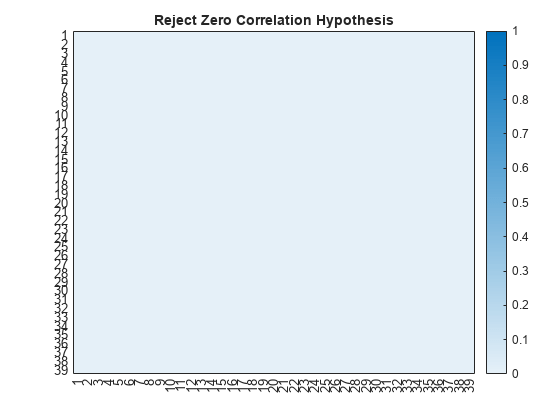
Specify a significance level of 0.05. For multiple comparisons, use the Bonferroni correction to test the hypothesis that the pairwise correlations between any two principal component features is zero. If for a given pair of features, p is less than the significance divided by the correction, then reject the hypothesis that those features have zero correlation. Plot the surface showing pairs of principal component features that reject the hypothesis of zero correlation.

    pvalue = 0.05;
    numFeatures = size(p,1);

    bonferroniCorrection = numFeatures*(numFeatures-1)/2;
    rejectZeroCorrHypotheses = p < pvalue / bonferroniCorrection;

    figure
    heatmap(single(rejectZeroCorrHypotheses),GridVisible="off",ColorLimits=[0,1],Title="Reject Zero Correlation Hypothesis")

In this example, the hypothesis that no correlation exists between any two features is not rejected.

end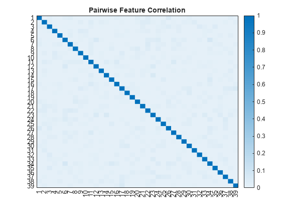

Test OOD Data Discriminator

Test the performance of the discriminator on the augmented training data.

XTrain = convertToDlarray(dsTrain,numObservationsTrain);

Generate OOD data sets by augmenting each training image.

XTrainLRFlip = fliplr(XTrain);
XTrainUDFlip = flipud(XTrain);
XTrainInvert = 1-XTrain;

Find the distribution scores for each of the data sets using the discriminator.

scoresTrain= distributionScores(discriminator,XTrain);
scoresTrainLRFlip = distributionScores(discriminator,XTrainLRFlip);
scoresTrainUDFlip = distributionScores(discriminator,XTrainUDFlip);
scoresTrainInvert = distributionScores(discriminator,XTrainInvert);

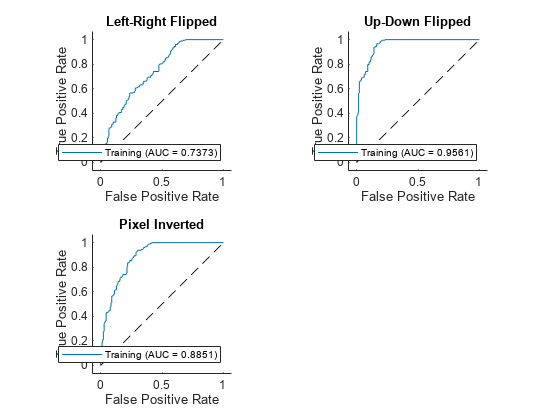
Find the receiver operating characteristic (ROC) curves for the original and augmented data sets using the discriminator and the distribution scores. A well-performing discriminator achieves an AUC value close to 1, corresponding to the discriminator being able to separate the ID and OOD data.

trueDataLabels = [
    repelem("Training",numObservationsTrain), ...
    repelem("Augmented",numObservationsTrain)];

scoresTrainAndLRFlip = [scoresTrain',scoresTrainLRFlip'];
scoresTrainAndUDFlip = [scoresTrain',scoresTrainUDFlip'];
scoresTrainAndInvert = [scoresTrain',scoresTrainInvert'];

rocObjTrainLRFlip = rocmetrics(trueDataLabels,gather(scoresTrainAndLRFlip),"Training");
rocObjTrainUDFlip = rocmetrics(trueDataLabels,gather(scoresTrainAndUDFlip),"Training");
rocObjTrainInvert = rocmetrics(trueDataLabels,gather(scoresTrainAndInvert),"Training");

Plot the ROC curves. If the discriminator performs well, then the ROC curve should be close to the top-left corner (corresponding to an AUC value of 1). The ROC curves show that the discriminator can distinguish the augmented images (OOD) from the training images (ID). The discriminator has greatest difficulty distinguishing the left-right flipped images as OOD. This is because those images are closer to the distribution of the training images. To ensure the model is robust to these augmentations, retrain the model using the augmented images. For more information, see Object Detection Using YOLO v4 Deep Learning (Computer Vision Toolbox).

figure
tiledlayout(2,2)
nexttile
plot(rocObjTrainLRFlip,ShowModelOperatingPoint=false)
title("Left-Right Flipped")
nexttile
plot(rocObjTrainUDFlip,ShowModelOperatingPoint=false)
title("Up-Down Flipped")
nexttile
plot(rocObjTrainInvert,ShowModelOperatingPoint=false)
title("Pixel Inverted")

The discriminator selects a threshold that best splits the ID and OOD data. Use the isInNetworkDistribution function to see the proportion of images classified as OOD by the discriminator. The function returns 1 (true) if the discriminator classifies the image as ID and 0 (false) if the discriminator classifies the image as OOD.

Test the discriminator on the original training data.

tfTrain = isInNetworkDistribution(discriminator,XTrain);
propotionTrainID = sum(tfTrain)/numel(tfTrain)

propotionTrainID =

    0.9548

For the training data, the proportion of ID observations is above the true positive goal of 0.975 specified when creating the discriminator.

Test the discriminator on the augmented training data. Find the proportion of left-right flipped images that the network classifies as ID.

tfTrainLRFlip = isInNetworkDistribution(discriminator,XTrainLRFlip);
propotionTrainLRFlipID = sum(tfTrainLRFlip)/numel(tfTrainLRFlip)

propotionTrainLRFlipID =

    0.6102

Find the proportion of up-down flipped images that the network classifies as ID.

tfTrainUDFlip = isInNetworkDistribution(discriminator,XTrainUDFlip);
propotionTrainUDFlipID = sum(tfTrainUDFlip)/numel(tfTrainUDFlip)

propotionTrainUDFlipID =

    0.1638

Find the proportion of inverted images that the network classifies as ID.

tfTrainInvert= isInNetworkDistribution(discriminator,XTrainInvert);
propotionTrainInvertID = sum(tfTrainInvert)/numel(tfTrainInvert)

propotionTrainInvertID =

    0.3503

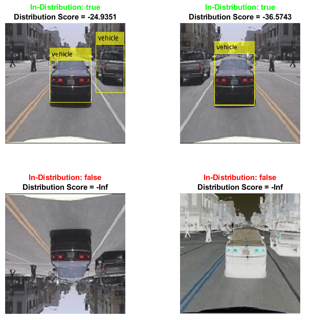
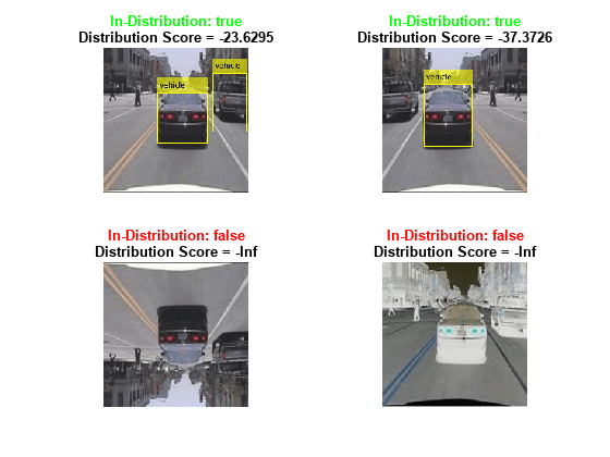
Visualize the results for the first image. The discriminator classifies the original training and the left-right flipped image as ID. The left-right flipped image is similar to the images that the network sees during training, so it is not surprising that the discriminator classifies this as ID. The left-right flipped image has a lower distribution confidence score reflecting the additional uncertainty. The up-down flipped and inverted images have a distribution score of -Inf. This is because those images are outside of the range of histograms that the HBOS method uses to compute the scores.

figure
tiledlayout(2,2)
nexttile
imshow(detectedImage)
colorTitle(tfTrain(1),scoresTrain(1))
nexttile
imshow(detectedLRFlip)
colorTitle(tfTrainLRFlip(1),scoresTrainLRFlip(1))
nexttile
imshow(detectedUDFlip)
colorTitle(tfTrainUDFlip(1),scoresTrainUDFlip(1))
nexttile
imshow(detectedInvert)
colorTitle(tfTrainInvert(1),scoresTrainInvert(1))

References

[1] Shalev, Gal, Gabi Shalev, and Joseph Keshet. “A Baseline for Detecting Out-of-Distribution Examples in Image Captioning.” In Proceedings of the 30th ACM International Conference on Multimedia, 4175–84. Lisboa Portugal: ACM, 2022. https://doi.org/10.1145/3503161.3548340.

[2] Markus Goldstein and Andreas Dengel. "Histogram-based outlier score (hbos): A fast unsupervised anomaly detection algorithm." KI-2012: poster and demo track 9 (2012).

Helper Functions

preprocessData

The preprocessData function takes as input data containing the image and the bounding box, and a target size, and returns the image and bounding box resized to match the target size.

function data = preprocessData(data,targetSize)
for num = 1:size(data,1)
    I = data{num,1};
    imgSize = size(I);
    bboxes = data{num,2};
    I = im2single(imresize(I,targetSize(1:2)));
    scale = targetSize(1:2)./imgSize(1:2);
    bboxes = bboxresize(bboxes,scale);
    data(num,1:2) = {I,bboxes};
end
end

preprocessMiniBatch

The preprocessMiniBatch function preprocesses a mini-batch of data by extracting the image data from the input cell array and concatenating the data into a numeric array.

function x = preprocessMiniBatch(xCell,~,~)
targetSize = [224 224 3];

for num = 1:size(xCell,1)
    I = xCell{num,1};
    I = im2single(imresize(I,targetSize(1:2)));
    xCell{num,1} = I;
end

% Concatenate over batch.
x = cat(4,xCell{:});
end

convertToDlarray

The convertToDlarray function takes as input a datastore and returns the data as a dlarray object.

function X = convertToDlarray(ds,numObservations)

minibatchsize = numObservations;
numOutputs = 1;

mbq = minibatchqueue(ds,numOutputs,...
    MiniBatchSize=minibatchsize,...
    MiniBatchFcn=@preprocessMiniBatch, ...
    OutputAsDlarray=ones(1,numOutputs), ...
    MiniBatchFormat="SSCB");

X = next(mbq);
end

plotAugmentedImages

Th plotAugmentedImages function takes as input four pairs of images (x, y, z, and w) and image titles (xtitle, ytitle, ztitle, and wtitle) and returns a plot.

function plotAugmentedImages(x,xtitle,y,ytitle,z,ztitle,w,wtitle)
tiledlayout(2,2)
nexttile
imshow(x)
title(xtitle)
nexttile
imshow(y)
title(ytitle)
nexttile
imshow(z)
title(ztitle)
nexttile
imshow(w)
title(wtitle)
end

colorTitle

The colorTitle function takes as input a logical value indicating if the image is ID, and the raw score, and returns a custom figure title.

function colorTitle(tf,score)
if gather(tf)
    title({"\color{green}" + "In-Distribution: " + gather(tf) + "\color{black}"; "Distribution Score = " + gather(score)})
else
    title({"\color{red}" + "In-Distribution: " + gather(tf) + "\color{black}"; "Distribution Score = " + gather(score)})
end
end

principalComponentFeatureCorrelation

The principalComponentFeatureCorrelation function takes as input a discriminator object and ID data and returns a matrix of the pairwise correlation coefficient between each pair of features and the p-values.

function [rho,p] = principalComponentFeatureCorrelation(discriminator,X)

layerName = discriminator.LayerNames;
features = predict(discriminator.Network,X,Outputs=layerName);

% Flatten the SSC channels.
nonBatchDims = [finddim(features,"S") finddim(features,"C")];
batchDim = finddim(features,"B");
sz = size(features);
features = reshape(extractdata(gather(features)), ...
    [prod(sz(nonBatchDims)),prod(sz(batchDim))]);

features = features';

% Compute the principal components.
[coeff,~,latent] = pca(features);
rank = sum( latent/max(latent) > discriminator.VarianceCutoff);
principalComponentFeatures = features*coeff(:,1:rank);

% Compute Kendall tau rank coefficients and pvalues.
[rho,p] = corr(principalComponentFeatures,Type="Kendall");
end