Multiloop Control Design for VTOL UAV in Fixed Wing Flight

Getting Started

To open the example livescript and directory which contains the Simulink project file, first run openExample('uav/TuneControlDesignForUAVInFixedWingFlightExample') in the command window.

You must open the VTOLRefApp.prj project file to access the Simulink model, supporting files, and project shorcuts that this example uses.

% Open the Simulink project after running openExample('uav/TuneControlDesignForUAVInFixedWingFlightExample')
prj = openProject("VTOLApp/VTOLRefApp.prj");

Warning: Unable to find configuration set 'VTOLConfiguration' for the active configuration reference 'Reference'

Use the highlighted project shortcuts for setting up the transition configuration. You can use the other project shortcuts for tuning the hover, transition configurations, and setting up the photorealistic city mission. To see these shortcuts, you must open and view the Project shortcuts tab.

To set up the aircraft plant model and base controller, click the Getting Started button in the project shortcuts or run the setupPlant helper function.

setupPlant;

Initialized VTOL model.
Enabled hover configuration.
Enabled hover guidance mission.

Setup Fixed Wing Configuration

To configure the UAV to fixed wing configuration, click the Set Fixed Wing Configuration shortcut or run the setupFixedWingConfiguration helper function.

setupFixedWingConfiguration;

Enabled fixed-wing configuration.

Setup Guidance Test Bench for Fixed Wing.

The fixed-wing controller must be robust and be able to track trajectories precisely so that the VTOL UAV can navigate in dense urban scenarios. Leverage guidance algorithms in UAV toolbox as a guidance-testbench to validate VTOL aircraft flying complex missions.

To set up a fixed wing mission, click Guidance Mode under the Fixed Wing section of Project Shortcuts, or run the setupFixedWingGuidanceMission helper function.

setupFixedWingGuidanceMission;

Enabled fixed-wing guidance mission.

Run the Simulink model and store the output in out by running the sim function as follows. To visualize the trajectory, open the UAV Animation block inside the Visualization subsystem. The UAV takes off and navigates through a few waypoints before reducing altitude and then orbiting around a reference point.

open_system(mdl);
out = sim(mdl);

Analyze Tracking and Control Performance with Untuned Gains

After executing the fixed wing mission, you can visualize the output UAV state to evaluate the control design performance.

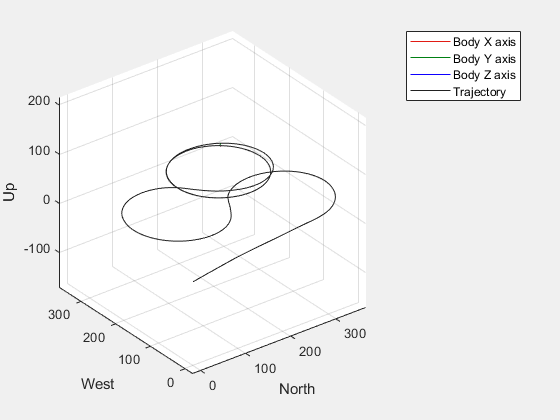
To plot the simulation ouput that you have stored in out, use the exampleHelperPlotFixedWingControlTrackingResults helper function. This allows you to visualize the control design performance by comparing the airspeed, altitude, pitch, roll, and position commands with their respective outputs.

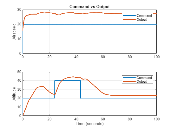
Observe the commanded altitude and airspeed with the output altitude and airspeed for the entire duration of the mission. The plots show that there is a significant steady state error in both measurements, and the UAV takes a long time to reduce its altitude.

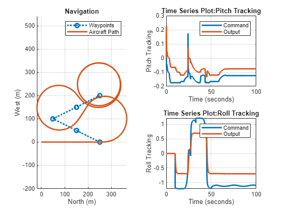
The third plot shows the navigation metrics of the UAV as it follows the commanded course. The plots are the aircraft path and the mission waypoints in the XY plane (left), and the comparisons of the pitch and roll angle output with the commanded values (right). The untuned controller is unable to track the reference angles, leading to the aircraft not able to efficiently navigate through the waypoints. The pitch controller performance also causes oscillatory behavior as shown in the altitude tracking plot.

exampleHelperPlotFixedWingControlTrackingResults(out,FixedWingMission)

Automate Tuning of Attitude Controller for Tiltrotor in Fixed Wing

In this step, you adjust the controller gains based on design goals specified for multiple feedback loops of the VTOLTiltrotor model by using systune (Simulink Control Design), a fixed-structure tuning method in Simulink® Control Design™ software.

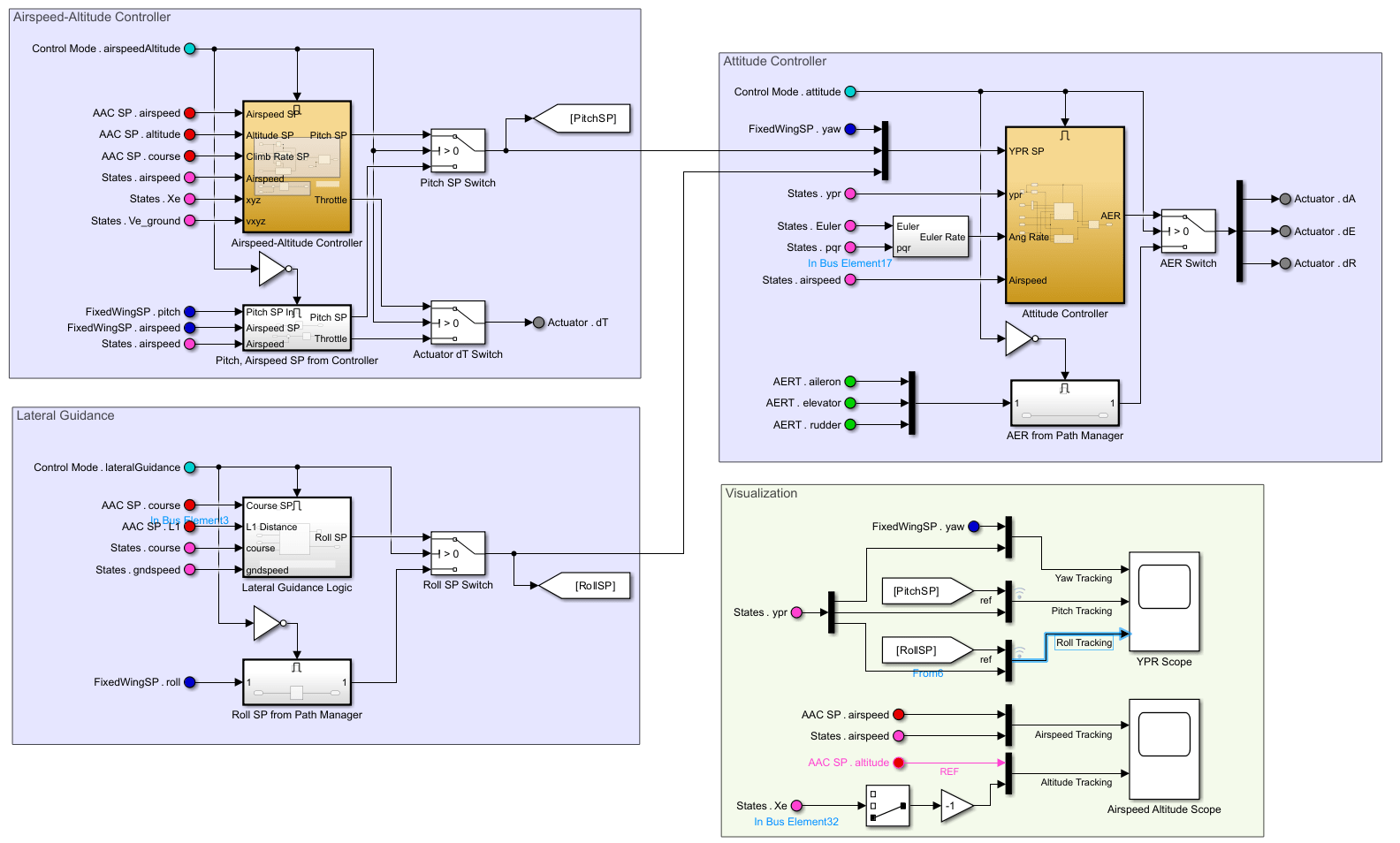
The Fixed Wing Controller subsystem in the model contains an inner loop Attitude Controller subsystem that tracks the roll and pitch angles. The outer loops of Airspeed-Altitude Controller and Lateral Guidance Logic subsystems compute the pitch and roll angular set points for the inner loop controller.

In this example, you use programmatic tuning for PID controllers in the attitude, altitude, and airspeed loops shown in the highlighted subsystems in the following diagram.

The desired response for the different loops is based on analysis that mentions settling time for the airspeed, altitude and roll controllers [4]. To obtain a faster response for the inner loops, you tune the pitch and roll control loop to a higher bandwidth.

Create Interface for Control Tuning

To tune the aircraft controllers, you must specify the angle setpoints, measured outputs, and the loop gain locations for pitch and roll loops as the linear analysis points.

To specify the analysis points and blocks to tune for pitch and roll loops, run the exampleHelperSetupFixedWingControlTuning_Attitude script.

exampleHelperSetupFixedWingControlTuning_Attitude;

Create an slTuner (Simulink Control Design) object, the interface for tuning of Simulink® models, using the controller blocks to tune and the analysis points as input. During tuning, the interface linearizes the model around an initial condition at which the aircraft is cruising in steady state with a fixed velocity.

options=slTunerOptions('AreParamsTunable',false);
attitudeTuner=slTuner(mdl,tunedBlocks,analysisPoints,options);
attitudeTuner.Ts=0.005;
attitudeTuner.OperatingPoints=5;

Create Tuning Goals for Pitch and Roll Controllers

Use loop-shaping design to create a desired open-loop response of an integrator. Set bandwidth to 20 rad/s for roll and 15 rad/s for pitch control loops. This helps track the reference inputs with zero steady state error, while attenuating inputs with frequencies that exceed the bandwidth.

wcRoll = 20;
wcPitch = 15;

Create the loop-shaping goals for the roll and pitch loops using TuningGoal.LoopShape (Control System Toolbox).

rollLoopShape = TuningGoal.LoopShape({rollOpenLoopLocation}, wcRoll);
rollLoopShape.Name = 'Roll Loop Shape';
pitchLoopShape = TuningGoal.LoopShape({pitchOpenLoopLocation}, wcPitch);
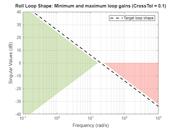
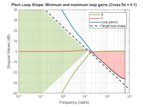
pitchLoopShape.Name = 'Pitch Loop Shape';

Visualize the loop shaping goal. The plot shows the singular values of the desired target loop shape. The green region shows the constraints on the inverse sensitivity function as minimum low-frequency loop gain, and the red region marks the complementary sensitivity as maximum high-frequency loop gain.

viewGoal(rollLoopShape);

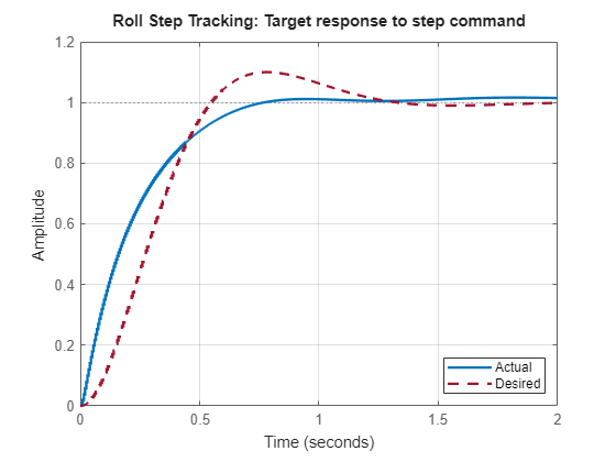
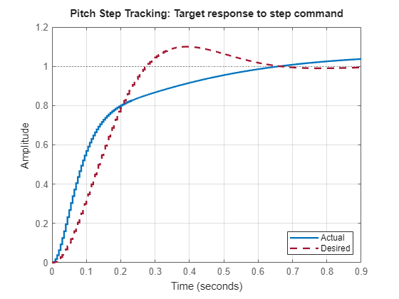
Create the tuning goals to match the step response to a desired first order response with a time constant of 0.1 seconds for pitch and 0.2 seconds for roll (see TuningGoal.StepTracking (Control System Toolbox)). These time constants map to the settling times mentioned in [4].

% Define time constant
tauRoll = 0.2;
tauPitch = 0.1;

To compute the linearized closed-loop response, compute the open loop response of the outer loops that compute the set points for pitch and roll.

% Roll Loop
rollStepTracking = TuningGoal.StepTracking({rollAngleInput},{rollAngleOutput}, tauRoll, 10);
rollStepTracking.Openings = [{rollAngleInput}; {pitchAngleInput}];
rollStepTracking.Name = 'Roll Step Tracking';

% Pitch Loop
pitchStepTracking = TuningGoal.StepTracking({pitchAngleInput},{pitchAngleOutput}, tauPitch, 10);
pitchStepTracking.Openings = [{rollAngleInput}; {pitchAngleInput}];
pitchStepTracking.Name = 'Pitch Step Tracking';

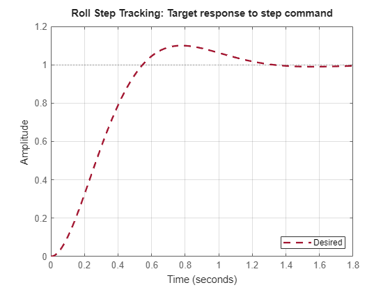
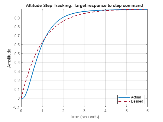
Visualize desired step response of the closed-loop system.

viewGoal(rollStepTracking);

Tune Controller Gains and Analyze Results

Use systune to tune the gains based on the defined soft goals.The systune function performs a multi-objective optimization to meet step tracking and frequency response requirements. Tuning for step tracking and loop shape tuning goals enables the controller to achieve a good tracking performance with a desired bandwidth that rejects of high frequency disturbance and noise.

% Options
options = systuneOptions();
options.Display = 'final';

% Tune
attitudeTuner_Tuned= systune(attitudeTuner,[rollLoopShape; rollStepTracking; pitchLoopShape; pitchStepTracking],options);

Final: Soft = 4.26, Hard = -Inf, Iterations = 29

Warning: Tuning goal "Roll Step Tracking": Feedback configuration has fixed integrators that cannot be stabilized with available tuning parameters. Make sure these are modeling artifacts rather than physical instabilities.

The best achieved soft constraint value of slightly greater than 1 indicates that the solution nearly satisfies all requirements. A closer inspection of the tuning goal plots shows that the multi-objective optimization returns a solution that matches the open loop shape and is slightly higher than desired bandwidth, as well as the closed-loop step response. This is considered acceptable for the inner loop performance as it nearly meets all the requirements of minimum and maximum loop gains and the overall objective is close to 1.

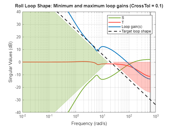
Visualize the loop shape and step response after the controller is tuned.

exampleHelperViewTuningGoal([rollLoopShape,rollStepTracking,pitchLoopShape,pitchStepTracking],attitudeTuner_Tuned);

Update Parameters

Update the VTOL UAV parameters with the tuned values. In this example, the exampleHelperWriteBlockValue_Attitude function updates the variable values in the MATLAB® workspace that the controller blocks uses. This function updates the FWControlParams struct in the workspace with the new control gains.

FWControlParams=exampleHelperWriteBlockValue_Attitude(attitudeTuner_Tuned,FWControlParams);

Automate Tuning of Airspeed-Altitude Controller for Tiltrotor in Fixed Wing

In this section, you tune the airspeed and altitude controllers using systune and slTuner, similar to tuning the attitude loops in the preceding section.

Define Interface for Tuning

Specify analysis points and blocks to tune for altitude and airspeed loops.

exampleHelperSetupFixedWingControlTuning_AltitudeAirspeed;

Create the slTuner object.

options = slTunerOptions('AreParamsTunable',false);
altitudeAirspeedTuner = slTuner(mdl,tunedBlocks,analysisPoints,options);
altitudeAirspeedTuner.Ts = 0.005;
altitudeAirspeedTuner.OperatingPoints = 5;

Create Tuning Goals for Altitude and Airspeed Controllers

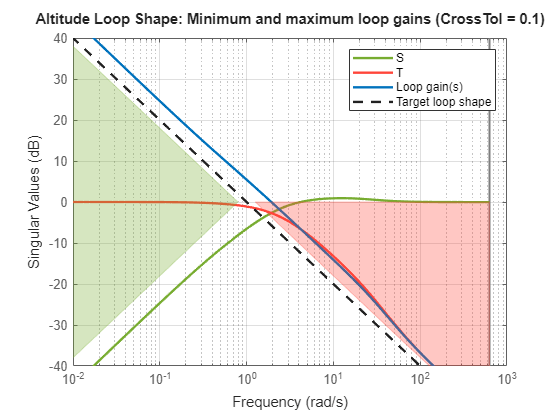
Create the desired loop shapes of an integrator with bandwidth of 1 rad/s for altitude control loop and 10 rad/s for airspeed control.

% Altitude Loop
Wc = 1;
altitudeLoopShape = TuningGoal.LoopShape({altitudeOpenLoopLocation},Wc);
altitudeLoopShape.Name = 'Altitude Loop Shape';
% Airspeed Loop
Wc = 10;
airspeedLoopShape = TuningGoal.LoopShape({airspeedOpenLoopLocation},Wc);
airspeedLoopShape.Name = 'Airspeed Loop Shape';

Create step tracking goals using first order response with time constants of 1 seconds for altitude and 0.1 seconds for airspeed.

% Altitude Loop
Tau = 1;
altitudeStepTracking = TuningGoal.StepTracking({altitudeInput},{altitudeOutput},Tau);
altitudeStepTracking.Name = 'Altitude Step Tracking';
% Airspeed Loop
Tau=0.1;
airspeedStepTracking = TuningGoal.StepTracking({airspeedInput},{airspeedOutput},Tau);
airspeedStepTracking.Name = 'Airspeed Step Tracking';

Tune Controller Gains and Analyze Results

Use systune to tune the gains based on the defined soft goals.

% Options
options = systuneOptions();
options.Display = 'final';

% Tune
[altitudeAirspeedTuner_Tuned] = systune(altitudeAirspeedTuner,[altitudeLoopShape; altitudeStepTracking; airspeedLoopShape; airspeedStepTracking],options);

Final: Soft = 1.74, Hard = -Inf, Iterations = 41

Compare the controller loop shape and step response after tuning to the tuning goals. The plots show that the tuned controllers are able to provide the required bandwidth and step tracking time response.

exampleHelperViewTuningGoal([altitudeLoopShape; altitudeStepTracking; airspeedLoopShape; airspeedStepTracking],altitudeAirspeedTuner_Tuned);

Update Parameters

Update the parameters with the tuned value by using the exampleHelperWriteBlockValue_AltitudeAirspeed. This function updates the variable values in the MATLAB® workspace used by the controller blocks in the model.

FWControlParams=exampleHelperWriteBlockValue_AltitudeAirspeed(altitudeAirspeedTuner_Tuned,FWControlParams);

Analyze Tracking and Control Performance with Tuned Gains

Disable the tuning mode and enable the test mode to set up the fixed wing guidance mission.

TestMode = 1;
TuningMode = 0;
setupFixedWingGuidanceMission;

Enabled fixed-wing guidance mission.

Run the Simulink model and store the output in out by running the sim function.

out = sim(mdl);

The altitude and airspeed plots show that the outputs converge in a shorter time without any steady state error and oscillations.

exampleHelperPlotFixedWingControlTrackingResults(out,FixedWingMission);

The comparison of pitch and roll angles shows an improved tracking with a faster response.This shows that the UAV navigates the waypoints more efficiently. Also, note that the roll tracking is saturated within the roll controller.

Summary

In this example, you have tuned the control design of a VTOL in fixed wing configuration.

Similar to the Tune Hover Control Design for VTOL UAV in Steady Wind Condition example, you can refine the gains that you have obtained for fixed-wing flight in steady wind condition by completing the following steps:

Next, design the control system of the transition mode of the VTOL UAV.

References

[1] N., Pavan. (2020). Design of Tiltrotor VTOL and Development of Simulink Environment for Flight Simulations.

[2] Mathur, Akshay & Atkins, Ella. (2021). Design, Modeling and Hybrid Control of a QuadPlane.

[3] Ducard, Guillaume Jacques Joseph and Minh-Duc Hua (2014). Modeling of an unmanned hybrid aerial vehicle.

[4] Transition from Low- to High-Fidelity UAV Models in Three Stages - The Mathworks Inc.

References

[1] N., Pavan. "Design of Tiltrotor VTOL and Development of Simulink Environment for Flight Simulations." Master's thesis, Indian Institute of Technology Madras, 2020.
[2] Mathur, Akshay, and Ella M. Atkins. "Design, Modeling and Hybrid Control of a QuadPlane." In AIAA Scitech 2021 Forum. VIRTUAL EVENT: American Institute of Aeronautics and Astronautics, 2021. https://doi.org/10.2514/6.2021-0374.
[3] Ducard, Guillaume, and Minh-Duc Hua. "Modeling of an Unmanned Hybrid Aerial Vehicle." In 2014 IEEE Conference on Control Applications (CCA), 1011–16. Juan Les Antibes, France: IEEE, 2014. https://doi.org/10.1109/CCA.2014.6981467.