cwtmag2sig

Signal reconstruction from CWT magnitude

Since R2023b

collapse all in page

Syntax

x = cwtmag2sig(cfs)

x = cwtmag2sig(cfs,fs)

x = cwtmag2sig(cfs,ts)

x = cwtmag2sig(___,Name=Value)

[x,t] = cwtmag2sig(___)

[x,t,info] = cwtmag2sig(___)

Description

x = cwtmag2sig(cfs) returns a time-domain real-valued signal x estimated from the continuous wavelet transform (CWT) magnitude, cfs, using the gradient descent method and the limited-memory Broyden–Fletcher–Goldfarb–Shanno (L-BFGS) optimizer. By default, cwtmag2sig uses the Morse (3,60) wavelet with default frequency range. The function assumes:

The CWT magnitude was obtained from a real-valued signal.
The ExtendSignal of the original CWT is false or the Boundary of the cwtfilterbank object used in the original CWT is "periodic".

To use the cwtmag2sig function, you must have a Deep Learning Toolbox™ license.

x = cwtmag2sig(cfs,fs) specifies the sample rate.

x = cwtmag2sig(cfs,ts) specifies the sample period.

x = cwtmag2sig(___,Name=Value) specifies additional options using name-value arguments. Options include, among others, the analytic wavelet to use in the reconstruction and the method to specify initial phases. These arguments can be added to any of the previous input syntaxes. For example, Wavelet="bump",InitializePhaseMethod="random" specifies that the signal is estimated using the bump wavelet with random initial phases.

For optimal reconstruction results, the sample rate and the values of the CWT Parameters must be consistent with those used to obtain the CWT magnitude. Also, retain and reuse the scaling coefficients obtained from the original CWT.

example

[x,t] = cwtmag2sig(___) also returns the times instants at which the signal is reconstructed.

[x,t,info] = cwtmag2sig(___) also returns a structure that contains information about the reconstruction process.

Examples

collapse all

Reconstruct Sinusoid from CWT Magnitude

This example uses:

Open Live Script

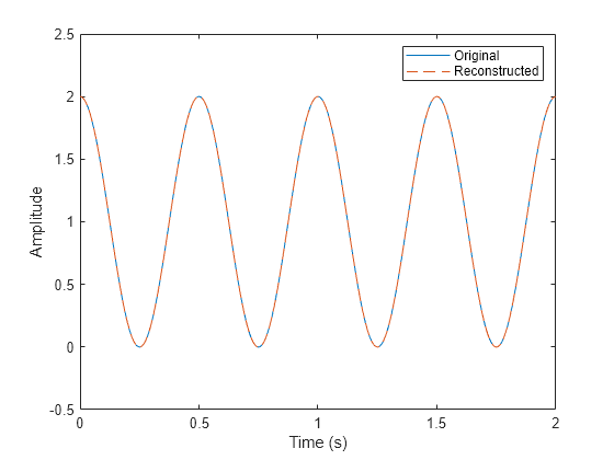
Consider a sinusoid with a frequency of 2 Hz and a DC value of 1. Sample the signal at 1000 Hz. Compute the CWT of the signal. In the CWT, do not extend the signal symmetrically. Also obtain the scaling coefficients of the transform.

fs = 1000;
ts = 0:1/fs:2-1/fs;
x = cos(2*pi*2*ts).'+1;
[CFS,~,~,~,scalcfs] = cwt(x,ExtendSignal=false);

Reconstruct the sinusoid from the magnitude of the CWT. Display the normalized inconsistency during the reconstruction process.

 xrec = cwtmag2sig(abs(CFS),...
     Display=true,ScalingCoefficients=scalcfs);

#Iteration  |  Normalized Inconsistency  
      1     |  1.6552e+00 
     20     |  2.5206e-03 
     40     |  6.9620e-03 
     60     |  7.6927e-04 
     67     |  1.5159e-06 

Decomposition process stopped.
The normalized inconsistency for each channel is smaller than the "InconsistencyTolerance" of 1e-05.

Plot the original and reconstructed signals.

 plot(ts,x,ts,xrec,"--")
 xlabel("Time (s)")
 ylabel("Amplitude")
 legend("Original","Reconstructed")

Figure contains an axes object. The axes object with xlabel Time (s), ylabel Amplitude contains 2 objects of type line. These objects represent Original, Reconstructed.

Use CWT Filter Bank to Reconstruct Multichannel Signal from CWT Magnitude

This example uses:

Open Live Script

Load an ECG signal corresponding to record 200 of the MIT-BIH Arrhythmia Database. Extract two segments, each with 1000 samples, from the signal. The workspace variable tm contains the sample times.

load mit200
idx1 =  1:1000;
idx2 = 3001:4000;
x1 = ecgsig(idx1);
x2 = ecgsig(idx2);

Create a CWT filter bank that you can use on the segments. Specify periodic boundary handling. Use the filter bank to obtain the CWT of the segments. Also obtain the scaling coefficients.

cfb = cwtfilterbank(SignalLength=length(x1), ...
    Boundary="periodic");
[CFS1,~,~,~,d1]  = cwt(x1,Filterbank=cfb);
[CFS2,~,~,~,d2]  = cwt(x2,Filterbank=cfb);

Concatenate the CWT coefficients along the third dimension. Also concatenate the scaling coefficients along the third dimension. Concatenate the segments along the second dimension. Treat each segment as a separate channel in a multichannel signal.

CFS = cat(3,CFS1,CFS2);
d = cat(3,d1,d2);
x = cat(2,x1,x2);

Use the filter bank to reconstruct the multichannel signal from the magnitudes of the CWT. Display the normalized inconsistency during the reconstruction process.

xrec = cwtmag2sig(abs(CFS),Display=true, ...
    ScalingCoefficients=d,Filterbank=cfb);

#Iteration  |  Normalized Inconsistency  
      1     |  1.6683e+00 1.6607e+00 
     20     |  1.3074e-01 2.0297e-01 
     40     |  4.0472e-02 4.1970e-02 
     60     |  6.8938e-03 4.8925e-03 
     80     |  1.8965e-02 2.0714e-02 
    100     |  5.7284e-02 3.3896e-02 
    120     |  4.1591e-02 1.3019e-02 
    140     |  5.0762e-02 5.6419e-03 
    160     |  1.9428e-02 3.9582e-04 
    180     |  1.9712e-03 2.5361e-05 
    200     |  2.9577e-04 5.7740e-06 
    220     |  1.1951e-05 5.7740e-06 
    222     |  9.2158e-06 5.7740e-06 

Decomposition process stopped.
The normalized inconsistency for each channel is smaller than the "InconsistencyTolerance" of 1e-05.

Plot the original and reconstructed channels.

tiledlayout(2,1)
nexttile
plot(tm(idx1),x(:,1),tm(idx1),xrec(:,1),"--")
ylabel("Amplitude")
title("First Channel")
legend("Original","Reconstructed",Location="northoutside")
nexttile
plot(tm(idx2),x(:,2),tm(idx2),xrec(:,2),"--")
title("Second Channel")
ylabel("Amplitude")
xlabel("Time (s)")

Figure contains 2 axes objects. Axes object 1 with title First Channel, ylabel Amplitude contains 2 objects of type line. These objects represent Original, Reconstructed. Axes object 2 with title Second Channel, xlabel Time (s), ylabel Amplitude contains 2 objects of type line.

Input Arguments

collapse all

`cfs` — CWT magnitude
matrix | 3-D array

CWT magnitude, specified as a matrix or a 3-D array. cfs must correspond to a real-valued signal.

When cfs corresponds to a single-channel signal, specify cfs as a matrix, with time increasing across the columns and frequency decreasing down the rows.
When cfs corresponds to a multichannel signal, specify cfs as a 3-D array, where the third dimension corresponds to the channels.

Data Types: single | double

`fs` — Sample rate
scalar

Sample rate corresponding to x in hertz, specified as a positive scalar.

Data Types: single | double

`ts` — Sample period
scalar duration

Sample period corresponding to x, specified as a positive scalar duration. The sample rate is calculated as 1/ts.

Data Types: duration

Name-Value Arguments

Specify optional pairs of arguments as Name1=Value1,...,NameN=ValueN, where Name is the argument name and Value is the corresponding value. Name-value arguments must appear after other arguments, but the order of the pairs does not matter.

Example: Wavelet="amor",VoicesPerOctave=20,Optimizer="adam" specifies that the signal is estimated using the Morlet (Gabor) wavelet, 20 voices per octave, and the adaptive moment estimation (ADAM) optimizer.

CWT Parameters

collapse all

`FrequencyLimits` — Frequency limits
two-element scalar vector

Frequency limits used for reconstruction, specified as a two-element vector with positive strictly increasing entries.

The first element specifies the lowest peak passband frequency and must be greater than or equal to the product of the wavelet peak frequency in hertz and two time standard deviations divided by the signal length.
The second element specifies the highest peak passband frequency and must be less than or equal to the Nyquist frequency.

The base-2 logarithm of the ratio of the upper frequency limit, freqMax, to the lower frequency limit, freqMin, must be greater than or equal to 1/NV, where NV is the number of voices per octave:

log₂(freqMax/freqMin) ≥ 1/NV.

If you specify frequency limits outside the permissible range, cwtmag2sig truncates the limits to the minimum and maximum valid values.

Data Types: single | double

`PeriodLimits` — Period limits
two-element duration array

Period limits to use in the CWT, specified as a two-element duration array with strictly increasing positive entries.

The first element must be greater than or equal to 2 × ts, where ts is the sampling period.
The maximum period cannot exceed the signal length divided by the product of two time standard deviations of the wavelet and the wavelet peak frequency.

The base-2 logarithm of the ratio of the minimum period, minP, to the maximum period, maxP, must be less than or equal to -1/NV, where NV is the number of voices per octave:

log₂(pMin/pMax) ≤ -1/NV.

If you specify period limits outside the permissible range, cwtmag2sig truncates the limits to the minimum and maximum valid values.

Data Types: duration

`Wavelet` — Wavelet
`"morse"` (default) | `"amor"` | `"bump"`

Wavelet used for reconstruction, specified as "morse", "amor", or "bump". These strings specify the analytic Morse, Morlet (Gabor), and bump wavelet, respectively. The default wavelet is the analytic Morse (3,60) wavelet. To learn more about Morse wavelets, see Morse Wavelets.

Data Types: char | string

`VoicesPerOctave` — Number of voices per octave
`10` (default) | integer

Number of voices per octave used for reconstruction, specified as a positive integer between 1 and 48. The CWT scales are discretized using the specified number of voices per octave.

Data Types: single | double

`TimeBandwidth` — Time-bandwidth product of the Morse wavelet
`60` (default) | scalar greater than or equal to 3 and less than or equal to 120

Time-bandwidth product for the Morse wavelet used for reconstruction, specified as a positive scalar greater than or equal to 3 and less than or equal to 120. The symmetry (gamma) of the Morse wavelet is fixed at 3. This property is only valid when Wavelet is "morse".

You cannot specify both TimeBandwidth and WaveletParameters.

In the notation of Morse Wavelets, TimeBandwidth is P².

Data Types: single | double

`WaveletParameters` — Morse wavelet parameters
`[3,60]` (default) | two-element vector of scalars

Morse wavelet parameters used for reconstruction, specified as a two-element vector. The first element is the symmetry parameter (gamma), which must be greater than or equal to 1. The second element is the time-bandwidth product, which must be greater than or equal to gamma. The ratio of the time-bandwidth product to gamma cannot exceed 40. This property is only valid when Wavelet is "morse".

You cannot specify both WaveletParameters and TimeBandwidth.

Data Types: single | double

`FilterBank` — CWT filter bank
`cwtfilterbank` object

CWT filter bank used for reconstruction, specified as a cwtfilterbank object. The CWT filter bank must have Boundary="periodic". If you specify FilterBank, you cannot specify any other CWT parameters. All options for the computation of the CWT are defined as properties of the filter bank. For more information, see cwtfilterbank.

Low Frequency Information

collapse all

`ScalingCoefficients` — Scaling coefficients
vector | 3-D array

Scaling coefficients for reconstruction, specified as a vector or 3-D array. You can obtain the scaling coefficients as an optional output of the cwt function.

For a single-channel signal, specify the scaling coefficients as a real-valued vector that is the same length as the column size of cfs.
For a multichannel signal, concatenate the scaling coefficients of each channel along the third dimension, and specify the scaling coefficients as the resulting 3-D array.

You cannot specify both ScalingCoefficients and SignalMean.

Data Types: single | double

`SignalMean` — Signal mean
scalar | vector

Signal mean to add to the reconstruction, specified as a scalar or vector. If the signal mean is a vector, it must be the same length as the column size of the wavelet coefficient matrix cfs.

For a single-channel signal, specify the signal mean as a real-valued scalar.
For a multichannel signal, specify the signal mean as a real-valued vector, where the ith element of SignalMean is the mean of the ithe channel.

Because the CWT does not preserve the signal mean, the reconstructed signal is a zero-mean signal by default. Adding a non-zero mean to a frequency- or period-limited reconstruction adds a zero-frequency component to the reconstruction.

You cannot specify both SignalMean and ScalingCoefficients.

Data Types: single | double

Algorithm Parameters

collapse all

`InitializePhaseMethod` — CWT phase initialization
`"random"` (default) | `"zeros"`

CWT phase initialization, specified as "random" or "zeros". Specify only one of InitializePhaseMethod or InitialPhase.

"random" — The function initializes the CWT phases as random numbers distributed uniformly in the interval [–π, π].
"zeros" — The function initializes the CWT phases as zeros.

Data Types: char | string

`InitialPhase` — Initial CWT phases
matrix | 3-D array

Initial CWT phases, specified as a real numeric matrix or 3-D array. Elements of InitialPhase must be in the range [–π, π]. InitialPhase must have the same size as cfs. Specify only one of InitializePhaseMethod or InitialPhase.

Data Types: single | double

`MaxIterations` — Maximum number of optimization iterations
`300` (default) | positive integer

Maximum number of optimization iterations used in the reconstruction process, specified as a positive integer. The reconstruction process stops when the number of iterations is greater than MaxIterations.

Data Types: single | double

`InconsistencyTolerance` — Inconsistency tolerance of reconstruction process
`1e-5` (default) | positive scalar

Inconsistency tolerance of reconstruction process, specified as a positive scalar. The reconstruction process stops when the Normalized Inconsistency is lower than the tolerance.

Data Types: single | double

`Optimizer` — Optimizer used in the gradient descent method
`"lbfgs"` (default) | `"sgdm"` | `"adam"` | `"rmsprop"`

Optimizer used in the gradient descent method, specified as one of these:

"lbfgs" — Limited-memory Broyden–Fletcher–Goldfarb–Shanno (L-BFGS) optimizer
"sgdm" — Stochastic gradient descent with momentum (SGDM) optimizer
"adam" — Adaptive moment estimation (ADAM) optimizer
"rmsprop" — Root-mean-square propagation (RMSProp) optimizer

Data Types: char | string

`StepSize` — Step size for iterative updates
`0.01` (default) | positive scalar

Step size for iterative updates used in the gradient descent method, specified as a positive scalar. This argument is valid only when Optimizer is not "lbfgs".

Data Types: single | double

`Display` — Inconsistency display option
`false` or `0` (default) | `true` or `1`

Inconsistency display option, specified as a numeric or logical 1 (true) or 0 (false). If this option is set to true, cwtmag2sig displays the normalized inconsistency after every 20 optimization iterations. The function also displays stopping information at the end of the run.

Data Types: logical

Output Arguments

collapse all

`x` — Estimated time-domain signal
vector | matrix

Estimated time-domain signal, returned as a vector or a matrix.

`t` — Time instants
vector

Time instants at which the signal is reconstructed, returned as a vector. When a sample rate is provided, t is a numeric vector in seconds. When a sample time duration ts is provided, t is a duration array with the same unit as ts. t is a numeric vector in sample numbers if no time information is provided. The number of rows in x equals the length of t.

`info` — Reconstruction process information
structure

Reconstruction process information, returned as a structure containing these fields:

ExitFlag — Termination flag of each channel.
- A value of 0 indicates the algorithm stopped when it reached the maximum number of iterations.
- A value of 1 indicates the algorithm stopped when it met the relative tolerance.
For multichannel signals, ExitFlag is a vector.
NumIterations — Total number of iterations for each channel. For multichannel signals, NumIterations is a vector.
Inconsistency — Average relative improvement toward convergence between the last two iterations for each channel. For multichannel signals, Inconsistency is a vector.
ReconstructedCWT — Reconstructed CWT at the final iteration.
ReconstructedPhase — Reconstructed phase at the final iteration.

More About

collapse all

Normalized Inconsistency

Normalized inconsistency measures improvement toward convergence of the reconstruction process in successive optimization iterations.

Normalized inconsistency is defined as

$Inconsistency = \frac{‖ s_{est, i} - s_{est, i - 1} ‖}{cfs},$

where s_est,i is the complex CWT estimated at the ith iteration and the brackets denote the matrix norm.

cwtmag2sig uses the MATLAB^® function norm to compute matrix norms.

Tips

If the reconstruction is not satisfactory, set Display to true. Observe the inconsistency during iterations. If the inconsistency does not decrease, reduce StepSize for better reconstruction.
The L-BFGS algorithm generally requires the fewest iterations and yields the best reconstruction results. This optimizer automatically selects the step size for each iteration. However, particularly when processing batch data inputs, the computation speed can be slow. When you need to perform a large number of calculations quickly, other optimizers are recommended.

Extended Capabilities

GPU Arrays
Accelerate code by running on a graphics processing unit (GPU) using Parallel Computing Toolbox™.

The cwtmag2sig function fully supports GPU arrays. To run the function on a GPU, specify the input data as a gpuArray (Parallel Computing Toolbox). For more information, see Run MATLAB Functions on a GPU (Parallel Computing Toolbox).

Version History

Introduced in R2023b

cwtmag2sig

Syntax

Description

Examples

Reconstruct Sinusoid from CWT Magnitude

Use CWT Filter Bank to Reconstruct Multichannel Signal from CWT Magnitude

Input Arguments

`cfs` — CWT magnitude
matrix | 3-D array

`fs` — Sample rate
scalar

`ts` — Sample period
scalar duration

Name-Value Arguments

`FrequencyLimits` — Frequency limits
two-element scalar vector

`PeriodLimits` — Period limits
two-element duration array

`Wavelet` — Wavelet
`"morse"` (default) | `"amor"` | `"bump"`

`VoicesPerOctave` — Number of voices per octave
`10` (default) | integer

`TimeBandwidth` — Time-bandwidth product of the Morse wavelet
`60` (default) | scalar greater than or equal to 3 and less than or equal to 120

`WaveletParameters` — Morse wavelet parameters
`[3,60]` (default) | two-element vector of scalars

`FilterBank` — CWT filter bank
`cwtfilterbank` object

`ScalingCoefficients` — Scaling coefficients
vector | 3-D array

`SignalMean` — Signal mean
scalar | vector

`InitializePhaseMethod` — CWT phase initialization
`"random"` (default) | `"zeros"`

`InitialPhase` — Initial CWT phases
matrix | 3-D array

`MaxIterations` — Maximum number of optimization iterations
`300` (default) | positive integer

`InconsistencyTolerance` — Inconsistency tolerance of reconstruction process
`1e-5` (default) | positive scalar

`Optimizer` — Optimizer used in the gradient descent method
`"lbfgs"` (default) | `"sgdm"` | `"adam"` | `"rmsprop"`

`StepSize` — Step size for iterative updates
`0.01` (default) | positive scalar

`Display` — Inconsistency display option
`false` or `0` (default) | `true` or `1`

Output Arguments

`x` — Estimated time-domain signal
vector | matrix

`t` — Time instants
vector

`info` — Reconstruction process information
structure

More About

Normalized Inconsistency

Tips

Extended Capabilities

GPU Arrays
Accelerate code by running on a graphics processing unit (GPU) using Parallel Computing Toolbox™.

Version History

See Also

Topics

cwtmag2sig

Syntax

Description

Examples

Reconstruct Sinusoid from CWT Magnitude

Use CWT Filter Bank to Reconstruct Multichannel Signal from CWT Magnitude

Input Arguments

cfs — CWT magnitude matrix | 3-D array

fs — Sample rate scalar

ts — Sample period scalar duration

Name-Value Arguments

FrequencyLimits — Frequency limits two-element scalar vector

PeriodLimits — Period limits two-element duration array

Wavelet — Wavelet "morse" (default) | "amor" | "bump"

VoicesPerOctave — Number of voices per octave 10 (default) | integer

TimeBandwidth — Time-bandwidth product of the Morse wavelet 60 (default) | scalar greater than or equal to 3 and less than or equal to 120

WaveletParameters — Morse wavelet parameters [3,60] (default) | two-element vector of scalars

FilterBank — CWT filter bank cwtfilterbank object

ScalingCoefficients — Scaling coefficients vector | 3-D array

SignalMean — Signal mean scalar | vector

InitializePhaseMethod — CWT phase initialization "random" (default) | "zeros"

InitialPhase — Initial CWT phases matrix | 3-D array

MaxIterations — Maximum number of optimization iterations 300 (default) | positive integer

InconsistencyTolerance — Inconsistency tolerance of reconstruction process 1e-5 (default) | positive scalar

Optimizer — Optimizer used in the gradient descent method "lbfgs" (default) | "sgdm" | "adam" | "rmsprop"

StepSize — Step size for iterative updates 0.01 (default) | positive scalar

Display — Inconsistency display option false or 0 (default) | true or 1

Output Arguments

x — Estimated time-domain signal vector | matrix

t — Time instants vector

info — Reconstruction process information structure

More About

Normalized Inconsistency

Tips

Extended Capabilities

GPU Arrays Accelerate code by running on a graphics processing unit (GPU) using Parallel Computing Toolbox™.

Version History

See Also

Topics

`cfs` — CWT magnitude
matrix | 3-D array

`fs` — Sample rate
scalar

`ts` — Sample period
scalar duration

`FrequencyLimits` — Frequency limits
two-element scalar vector

`PeriodLimits` — Period limits
two-element duration array

`Wavelet` — Wavelet
`"morse"` (default) | `"amor"` | `"bump"`

`VoicesPerOctave` — Number of voices per octave
`10` (default) | integer

`TimeBandwidth` — Time-bandwidth product of the Morse wavelet
`60` (default) | scalar greater than or equal to 3 and less than or equal to 120

`WaveletParameters` — Morse wavelet parameters
`[3,60]` (default) | two-element vector of scalars

`FilterBank` — CWT filter bank
`cwtfilterbank` object

`ScalingCoefficients` — Scaling coefficients
vector | 3-D array

`SignalMean` — Signal mean
scalar | vector

`InitializePhaseMethod` — CWT phase initialization
`"random"` (default) | `"zeros"`

`InitialPhase` — Initial CWT phases
matrix | 3-D array

`MaxIterations` — Maximum number of optimization iterations
`300` (default) | positive integer

`InconsistencyTolerance` — Inconsistency tolerance of reconstruction process
`1e-5` (default) | positive scalar

`Optimizer` — Optimizer used in the gradient descent method
`"lbfgs"` (default) | `"sgdm"` | `"adam"` | `"rmsprop"`

`StepSize` — Step size for iterative updates
`0.01` (default) | positive scalar

`Display` — Inconsistency display option
`false` or `0` (default) | `true` or `1`

`x` — Estimated time-domain signal
vector | matrix

`t` — Time instants
vector

`info` — Reconstruction process information
structure

GPU Arrays
Accelerate code by running on a graphics processing unit (GPU) using Parallel Computing Toolbox™.