waveletPooling2dLayer

2-D discrete wavelet pooling layer

Since R2026a

Description

A 2-D discrete wavelet pooling layer applies the forward and inverse discrete wavelet transforms to reconstruct approximations of the layer input. Use this layer to downsample the layer input along the spatial dimensions. The layer supports learnable (adaptive) and nonadaptive pooling. For more information, see Discrete Wavelet Pooling. Use of this layer requires Deep Learning Toolbox™.

Creation

Syntax

layer = waveletPooling2dLayer

layer = waveletPooling2dLayer(PropertyName=Value)

Description

layer = waveletPooling2dLayer creates a 2-D discrete wavelet pooling layer. By default, the layer obtains the 2-D discrete wavelet transform (DWT) of the input down to level two using the Haar wavelet, then uses the lowpass and detail (wavelet) subbands at that level to construct a pooled output at level one. Because the layer supports learnable pooling and you can choose which detail coefficients to include in the pooling, the layer output may not equal the level-one lowpass coefficients of the DWT.

The input to waveletPooling2dLayer must be a real-valued dlarray (Deep Learning Toolbox) object in "SSCB" format. The output is a dlarray object in "SSCB" format. For more information, see Layer Output Format.

Note

When you initialize the learnable parameters of waveletPooling2dLayer, the layer weights are set to unity. It is not recommended to initialize the weights directly.

layer = waveletPooling2dLayer(PropertyName=Value) creates a wavelet pooling layer with properties specified by one or more name-value arguments. You can specify the boundary extension mode and the level of decomposition, among others.

Example: layer = waveletPooling2dLayer(Wavelet="db4",Boundary="zeropad") creates a wavelet pooling layer that uses the extremal phase Daubechies wavelet with four vanishing moments and zero padding at the boundaries.

example

Properties

expand all

DWT

`Wavelet` — Wavelet
`"haar"` or `"db1"` (default) | character vector | string scalar

This property is read-only after object creation.

Real-valued orthogonal or biorthogonal wavelet, specified as a string scalar or character vector recognized by wavemngr. The layer uses the specified wavelet in the 2-D DWT.

Data Types: char | string

`ReconstructionLevel` — Reconstruction level
`1` (default) | nonnegative integer

This property is read-only after object creation.

Reconstruction level, specified as a nonnegative integer between 0 and min(log2([size(X,1) size(X,2)])), where X is the layer input. The layer reconstructs the pooled output at level ReconstructionLevel. By default, the layer output is a factor-of-2 dimension reduction for each input feature.

If you set ReconstructionLevel, then the default value of AnalysisLevel is ReconstructionLevel+1.

For more information about the size of the layer output, see Layer Output Format.

Data Types: single | double

`AnalysisLevel` — Analysis level
`2` (default) | positive integer

This property is read-only after object creation.

Analysis level, or decomposition level, of the 2-D DWT, specified as a positive integer between 1 and min(log2([size(X,1) size(X,2)])), where X is the layer input. AnalysisLevel must be greater than ReconstructionLevel.

If you set AnalysisLevel, then the default value of ReconstructionLevel is AnalysisLevel−1.

Data Types: single | double

`Boundary` — Boundary extension mode
`"reflection"` (default) | `"periodic"` | `"zeropad"`

This property is read-only after object creation.

Boundary extension mode to use in the DWT, specified as "reflection", "periodic", or "zeropad". The layer extends the coefficients at the boundary at each decomposition level based on the corresponding mode in dwtmode:

"reflection" — Half-point symmetric extension, "sym"
"periodic" — Periodic extension, "per"
"zeropad — Zero padding, "zpd"

To learn how the boundary extension mode can affect the size of the layer output, see Layer Output Format.

`SelectedDetailCoefficients` — Mask indicating which detail coefficients to include in pooling
`true(1,3,AnalysisLevel-ReconstructionLevel)` (default) | array of logical values

This property is read-only after object creation.

Mask indicating which detail (wavelet) coefficients to include in pooling, specified as a logical array.

The shape of the array is Nchannel-by-3-by-Ndiff, where Nchannel is the number of channels in the layer input, 3 represents the three wavelet subbands in the order LH (horizontal details), HL (vertical details), and HH (diagonal details), and Ndiff is the difference between the analysis level and reconstruction level. The pages of the array correspond to the decomposition levels ordered from finer to coarser scale. The layer includes and excludes the detail coefficients for pooling when the corresponding value in the mask is 1 (true) or 0 (false), respectively.

If Nchannel is equal to 1 and the input to the layer's forward / predict object function has more than one channel, the layer expands the values of SelectedDetailCoefficients in the 1-by-3-by-Ndiff array to all channels.
If you set Ndiff to 1 and the difference between the analysis and reconstruction levels is greater than 1, the layer expands the SelectedDetailCoefficients values to all levels.

The following 1-D example illustrates how SelectedDetailCoefficients interacts with DetailWeights. The behavior is identical for the 2-D wavelet pooling layer. If SelectedDetailCoefficients = [1 0 1] and DetailWeights = [0.5 1e3 0.4], the layer applies only the first and third gains to the detail coefficients at the corresponding levels during pooling. Because the value of the mask corresponding to the middle level is 0, the coefficients at that level are ignored. The gain corresponding to the middle level is effectively zero.

Data Types: logical

`ExpectedOutputSize` — Expected size of layer output along spatial dimensions
`"none"` (default) | two-element vector

This property is read-only after object creation.

Expected size of the layer output along the spatial dimensions, specified as "none" or a two-element vector. By default, the output size is not verified. If you set ExpectedOutputSize and the output sizes do not match the specified value, the result is an error.

ExpectedOutputSize plays an analogous role to the bookkeeping matrix S output argument of wavedec2, when that information is missing. The bookkeeping matrix contains the dimensions of the coefficients by level and the dimensions of the input.

Parameters

`DetailWeights` — Detail (wavelet) coefficient subband weights
`[]` (default) | numeric array | `dlarray` object

Detail (wavelet) coefficient subband weights, specified as [], a numeric array, or a dlarray object.

These layer weights are learnable parameters. DetailWeights is a Nchannel-by-3-by-Ndiff tensor, where Nchannel is the number of channels in the layer input, 3 represents the three wavelet subbands in the order LH (horizontal details), HL (vertical details), and HH (diagonal details), and Ndiff is the difference between the analysis level and reconstruction level. You can use the function initialize (Deep Learning Toolbox) to initialize the learnable parameters of a deep learning neural network that includes waveletPooling2dLayer objects. When you initialize the layers, initialize sets DetailWeights to ones(Nchannel,3,AnalysisLevel-ReconstructionLevel).

You must initialize waveletPooling2dLayer before using the layer's forward/predict method.

Data Types: single | double

`LowpassWeights` — Lowpass (LL) coefficient subband weights
`[]` (default) | numeric array | `dlarray` object

Lowpass (scaling) coefficient subband weights, specified as [], a numeric array, or a dlarray object.

These layer weights are learnable parameters. LowpassWeights is a Nchannel-byNdiff tensor, where Nchannel is the number of channels in the layer input and Ndiff is the difference between the analysis level and reconstruction level. You can use the function initialize (Deep Learning Toolbox) to initialize the learnable parameters of a deep learning neural network that includes waveletPooling2dLayer objects. When you initialize the layers, initialize sets LowpassWeights to ones(Nchannel,AnalysisLevel-ReconstructionLevel).

You must initialize waveletPooling2dLayer before using the layer's forward/predict method.

It is not recommended to initialize the weights directly.

Data Types: single | double

Learning Rate

`DetailWeightLearnRateFactor` — Learning rate factor for detail (wavelet) coefficient subband weights
`0` (default) | nonnegative scalar

Learning rate factor for the detail (wavelet) coefficient subband weights, specified as a nonnegative scalar. By default, the weights do not update with training. You can also set this property using the function setLearnRateFactor (Deep Learning Toolbox).

To perform adaptive pooling, specify a nonzero learning rate factor. When DetailWeightLearnRateFactor is nonzero, the layer uses the detail subband weights to modify the wavelet coefficients.

Data Types: single | double

`LowpassWeightLearnRateFactor` — Learning rate factor for the lowpass (LL) coefficient subband weights
`0` (default) | nonnegative scalar

Learning rate factor for the lowpass (LL) coefficient subband weights, specified as a nonnegative scalar. By default, the weights do not update with training. You can also set this property using the function setLearnRateFactor (Deep Learning Toolbox).

To perform adaptive pooling, specify a nonzero learning rate factor. When LowpassWeightLearnRateFactor is nonzero, the layer uses the lowpass weights to modify the lowpass (scaling) coefficients.

Data Types: single | double

Layer

`Name` — Layer name
`''` (default) | character vector

Layer name, specified as a character vector. For Layer array input, the trainnet (Deep Learning Toolbox) and dlnetwork (Deep Learning Toolbox) functions automatically assign names to unnamed layers.

Data Types: char

`NumInputs` — Number of inputs
Read-only: `1` (default)

This property is read-only.

Number of inputs to the layer, stored as 1. This layer accepts a single input only.

Data Types: double

`InputNames` — Input names
Read-only: `{'in'}` (default)

This property is read-only.

Input names, stored as {'in'}. This layer accepts a single input only.

Data Types: cell

`NumOutputs` — Number of outputs
Read-only: `1` (default)

This property is read-only.

Number of outputs from the layer, stored as 1. This layer has a single output only.

Data Types: double

`OutputNames` — Output names
Read-only: `{'out'}` (default)

This property is read-only.

Output names, stored as {'out'}. This layer has a single output only.

Data Types: cell

Examples

collapse all

Use `waveletPooling2dLayer` in Deep Learning Network

This example uses:

Open Live Script

Load the xbox image. The image is a 128-by-128 matrix. Save the image in single precision as a dlarray object with format "SSCB".

load xbox
dlimg = dlarray(single(xbox),"SSCB");

Create the default 2-D discrete wavelet pooling layer. By default, the learnable parameters DetailWeights and LowpassWeights are both empty.

dwtPool = waveletPooling2dLayer

dwtPool = 
  waveletPooling2dLayer with properties:

                            Name: ''
     DetailWeightLearnRateFactor: 0
    LowpassWeightLearnRateFactor: 0
                         Wavelet: 'db1'
             ReconstructionLevel: 1
                   AnalysisLevel: 2
                        Boundary: 'reflection'
      SelectedDetailCoefficients: [1 1 1]
              ExpectedOutputSize: 'none'

   Learnable Parameters
                   DetailWeights: []
                  LowpassWeights: []

   State Parameters
    No properties.

  Show all properties

Include the default 2-D wavelet pooling layer in a Layer array.

layers = [ ...
    imageInputLayer([128 128 1])
    waveletPooling2dLayer]

layers = 
  2×1 Layer array with layers:

     1   ''   Image Input             128×128×1 images with 'zerocenter' normalization
     2   ''   waveletPooling2dLayer   waveletPooling2dLayer

Convert the layer array to a dlnetwork object. Because the layer array has an input layer and no other inputs, the software initializes the network.

dlnet = dlnetwork(layers)

dlnet = 
  dlnetwork with properties:

         Layers: [2×1 nnet.cnn.layer.Layer]
    Connections: [1×2 table]
     Learnables: [2×3 table]
          State: [0×3 table]
     InputNames: {'imageinput'}
    OutputNames: {'layer'}
    Initialized: 1

  View summary with summary.

Confirm the network learnable parameters are DetailWeights and LowpassWeights.

dlnet.Learnables

ans=2×3 table
     Layer        Parameter            Value    
    _______    ________________    _____________

    "layer"    "DetailWeights"     {1×3 dlarray}
    "layer"    "LowpassWeights"    {1×1 dlarray}

Inspect the wavelet pooling layer in the network. Confirm the software initialized the weights.

dlnet.Layers(2)

ans = 
  waveletPooling2dLayer with properties:

                            Name: 'layer'
     DetailWeightLearnRateFactor: 0
    LowpassWeightLearnRateFactor: 0
                         Wavelet: 'db1'
             ReconstructionLevel: 1
                   AnalysisLevel: 2
                        Boundary: 'reflection'
      SelectedDetailCoefficients: [1 1 1]
              ExpectedOutputSize: 'none'

   Learnable Parameters
                   DetailWeights: [1×3 dlarray]
                  LowpassWeights: [1×1 dlarray]

   State Parameters
    No properties.

  Show all properties

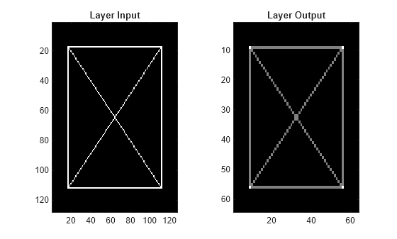
Run the image through the network. By default, the layer outputs the level-one lowpass approximation of the input.

dlnetout = forward(dlnet,dlimg);
size(dlnetout)

ans = 1×4

    64    64     1     1

dims(dlnetout)

ans = 
'SSCB'

Plot the layer input and output.

dlnetout2 = squeeze(extractdata(dlnetout));
tiledlayout(1,2)
nexttile
imagesc(xbox)
title("Layer Input")
nexttile
imagesc(dlnetout2)
title("Layer Output")
colormap gray

Figure contains 2 axes objects. Axes object 1 with title Layer Input contains an object of type image. Axes object 2 with title Layer Output contains an object of type image.

Recreate `waveletPooling2dLayer` Output Using `dldwt` and `dlidwt`

This example uses:

Open Live Script

Load the xbox image. The image dimensions are 128-by-128. Save the image in single precision as a dlarray object with format "SSCB".

load xbox
dlimg = dlarray(single(xbox),"SSCB");

Create a 2-D discrete wavelet pooling layer that uses the biorthogonal bior4.4 wavelet, which has four vanishing moments each for the decomposition and reconstruction filters. Set the analysis level to 4 and reconstruction level to 1. Set the boundary extension mode to "zeropad". Specify a mask so that the layer excludes from the pooling:

The LH subband (horizontal details) at level 3
The HL subband (vertical details) at level 2
The wavelet HH subband (diagonal details) at levels 3 and 4

% specify levels
alevel = 4;
rlevel = 1;
bdy = "zeropad";
wv = "bior4.4";

% create mask
msk = ones(1,3,alevel-rlevel);
msk(1,1,2) = 0;                % exclude LH subband
msk(1,2,1) = 0;                % exclude HL subband
msk(1,3,2:3) = 0;              % exclude HH subband


% create layer
poolDWT = waveletPooling2dLayer(AnalysisLevel=alevel, ...
    ReconstructionLevel=rlevel, ...
    SelectedDetailCoefficients=msk, ...
    Wavelet=wv, ...
    Boundary=bdy);

Create a Layer array containing an image input layer and the pooling layer.

layers = [ ...
    imageInputLayer([size(dlimg,1:2) 1])
    poolDWT];

Convert the layer array to a dlnetwork object.

dlnet = dlnetwork(layers);
dlnet.Layers(2)

ans = 
  waveletPooling2dLayer with properties:

                            Name: 'layer'
     DetailWeightLearnRateFactor: 0
    LowpassWeightLearnRateFactor: 0
                         Wavelet: "bior4.4"
             ReconstructionLevel: 1
                   AnalysisLevel: 4
                        Boundary: 'zeropad'
      SelectedDetailCoefficients: [1×3×3 double]
              ExpectedOutputSize: 'none'

   Learnable Parameters
                   DetailWeights: [1×3×3 dlarray]
                  LowpassWeights: [1×1 dlarray]

   State Parameters
    No properties.

  Show all properties

Run the signal through the network.

netout = forward(dlnet,dlimg);

Now use the same layer property values in the functions dldwt and dlidwt.

Use the dldwt function to obtain the differentiable DWT of the image down to level 4. To specify the extension mode, use the PaddingMode name-value argument. To obtain the full wavelet decomposition instead of only the final level wavelet coefficients, set the full wavelet decomposition option to true.

[A,D] = dldwt(dlimg, ...
    Wavelet=wv, ...
    Level=alevel, ...
    FullTree=true, ...
    PaddingMode=bdy);

For a multilevel 2-D inverse DWT, the dlidwt function expects the wavelet subband gains (mask) to be an NC-by-3-by-L matrix, where NC is the number of channels in the data, and L is the difference between the decomposition level (used to obtain the coefficients) and the reconstruction level. Use the dlidwt function to reconstruct the DWT up to level 2. Set the extension mode to zero padding and the DetailGain name-value argument to the mask.

dlout = dlidwt(A,D, ...
    Wavelet=wv, ...
    Level=rlevel, ...
    DetailGain=msk, ...
    PaddingMode=bdy);

Confirm the sizes of the layer output and dlidwt output are identical.

size(netout)

ans = 1×4

    68    68     1     1

size(dlout)

ans = 1×4

    68    68     1     1

Confirm the outputs are equal.

netoutEx = extractdata(netout);
dloutEx = extractdata(dlout);
max(abs(netoutEx(:)-dloutEx(:)))

ans = single

0

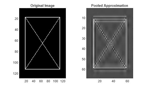
Plot the original image and its pooled approximation.

tiledlayout(1,2)
nexttile
imagesc(xbox)
axis tight
title("Original Image")
nexttile
imagesc(netoutEx)
axis tight
title("Pooled Approximation")
colormap gray

Figure contains 2 axes objects. Axes object 1 with title Original Image contains an object of type image. Axes object 2 with title Pooled Approximation contains an object of type image.

Determine Expected Output Size of 2-D Discrete Wavelet Pooling Layer

This example uses:

Open Live Script

Create a 127-by-135 image. Save the image in single precision as a dlarray object.

img = randn(127,135);
dlimg = dlarray(img,"SSCB");

The reconstruction level and the difference between the analysis and reconstruction levels can affect the output size.

Reconstruction Level Greater Than 0, Difference Between Analysis and Reconstruction Levels Greater Than 1

Use the dldwt function to obtain the differentiable DWT of the image down to level 4. Specify the db2 wavelet and zero padding as the extension mode. Obtain the full wavelet decomposition by setting FullTree to true.

wv = "db2";
alevel = 4;
bdy = "zeropad";

[A,D] = dldwt(dlimg, ...
    Wavelet=wv, ...
    Level=alevel, ...
    FullTree=true, ...
    PaddingMode=bdy); %#ok<*ASGLU>

Create a waveletPooling2dLayer using the same parameters as the dldwt function. Specify a reconstruction level of 2.

rlevel = 2;

wpl = waveletPooling2dLayer(Wavelet=wv, ...
    AnalysisLevel=alevel, ...
    ReconstructionLevel=rlevel, ...
    Boundary=bdy);

Create a Layer array containing an image input layer appropriate for the signal and the wavelet pooling layer. Convert the layer array to a dlnetwork object. Run the image through the network.

layers = [
    imageInputLayer([size(dlimg,1:2) 1])
    wpl];

dlnet = dlnetwork(layers);
netOutput = forward(dlnet,dlimg);

Compare the sizes of the spatial dimensions of the layer output with the dimensions of the coefficients at the corresponding decomposition level. Because the reconstruction level is greater than 0 and the difference between the analysis and reconstruction levels is greater than 1, the sizes are equal. The layer effectively sets FullTree to true which removes any ambiguity regarding the size of the reconstruction.

[size(netOutput,[1 2]); size(D{rlevel},[1 2])]

Reconstruction Level is 0

Use the dldwt function to obtain the differentiable DWT of the image down to level 2. Specify the db2 wavelet and zero padding as the extension mode. Set FullTree to true to obtain the full wavelet decomposition.

wv = "db2";
alevel = 2;
bdy = "zeropad";

[A,D] = dldwt(dlimg, ...
    Wavelet=wv, ...
    Level=alevel, ...
    FullTree=true, ...
    PaddingMode=bdy);

Use the dlidwt function to obtain the reconstruction at level 0. Compare the dimensions of the reconstruction with the dimensions of the original signal. Even though FullTree is true, the dimensions are different. Because the reconstruction level is 0, ambiguity exists.

rlevel = 0;

xrec = dlidwt(A,D, ...
    Wavelet=wv, ...
    Level=rlevel, ...
    PaddingMode=bdy);

[size(dlimg,[1 2]) ; size(xrec,[1 2])]

Because the reconstruction level is 0, the size of the reconstruction must equal the size of the original signal. You can set ExpectedOutputSize to remove the ambiguity.

xrec2 = dlidwt(A,D, ...
    Wavelet=wv, ...
    Level=rlevel, ...
    PaddingMode=bdy, ...
    ExpectedOutputSize=size(dlimg,[1 2]));

[size(dlimg,[1 2]) ; size(xrec2,[1 2])]

Similarly, to remove the ambiguity in the wavelet pooling layer, you can specify ExpectedOutputSize. Create a Layer array containing an image input layer and the wavelet pooling layer. Convert the layer array to a dlnetwork object. Run the image through the network.

wpl = waveletPooling2dLayer(Wavelet=wv, ...
    AnalysisLevel=alevel, ...
    ReconstructionLevel=rlevel, ...
    Boundary=bdy, ...
    ExpectedOutputSize=size(dlimg,[1 2]));

layers = [
    imageInputLayer([size(dlimg,[1 2]),1])
    wpl];
dlnet = dlnetwork(layers);
dlnetout = forward(dlnet,dlimg);

[size(dlimg,[1 2]) ; size(dlnetout,[1 2])]

Difference Between Analysis and Reconstruction Levels is 1

When the difference between the analysis and reconstruction levels is 1, the pooling layer behaves as if FullTree is false. Use the dldwt function to obtain the differentiable DWT of the image down to level 2. Specify the db2 wavelet and zero padding as the extension mode. Set FullTree to false.

wv = "db2";
alevel = 2;
bdy = "zeropad";

[A,D] = dldwt(dlimg, ...
    Wavelet=wv, ...
    Level=alevel, ...
    FullTree=false, ...
    PaddingMode=bdy);

If the input coefficients are a tensor, the dlidwt function performs a single-level IDWT. Obtain the size of the reconstruction.

xrec = dlidwt(A,D, ...
    Wavelet=wv, ...
    PaddingMode=bdy);
size(xrec,[1 2])

ans = 1×2

    66    70

Use the wavedec2 function to obtain the bookkeeping matrix of an image whose dimensions equal the size of the spatial dimensions of the dlarray object. Use the same input parameters. Use zero padding boundary extension. Extract from the bookkeeping matrix the sizes of the coefficients at level 2. Because FullTree is false, the sizes extracted from the bookkeeping matrix do not equal the sizes of the reconstruction.

origMode = dwtmode("status","nodisplay");
dwtmode("zpd","nodisplay")
[~,s] = wavedec2(img,alevel,wv);
dwtmode(origMode,"nodisplay")

extractedSize = s(end-2+1,:)

extractedSize = 1×2

    65    69

Use the dlidwt function to obtain the reconstruction at level 1, but this time specify ExpectedOutputSize to equal the extracted values.

xrec2 = dlidwt(A,D, ...
    Wavelet=wv, ...
    PaddingMode=bdy, ...
    ExpectedOutputSize=extractedSize);
size(xrec2,[1 2])

ans = 1×2

    65    69

Create a wavelet pooling layer. Set the layer properties to agree with the dldwt and dlidwt input arguments, including the expected output size. Create a Layer array containing an image input layer and the wavelet pooling layer. Convert the layer array to a dlnetwork object. Run the image through the network. Confirm the sizes of the network output equal ExpectedOutputSize.

rlevel = 1;

wpl = waveletPooling2dLayer(Wavelet=wv, ...
    AnalysisLevel=alevel, ...
    ReconstructionLevel=rlevel, ...
    Boundary=bdy, ...
    ExpectedOutputSize=extractedSize);

layers = [
    imageInputLayer([size(dlimg,[1 2]),1])
    wpl];
dlnet = dlnetwork(layers);
dlnetout = forward(dlnet,dlimg);

size(dlnetout,[1 2])

ans = 1×2

    65    69

More About

expand all

Discrete Wavelet Pooling

A discrete wavelet pooling layer performs downsampling by outputting the wavelet approximation at the specified level.

Williams and Li proposed a wavelet pooling scheme for convolutional-based networks [1]. The layer first obtains the DWT of the input down to level AnalysisLevel. The layer then uses the coarse-scale lowpass (scaling) coefficients and the detail coefficients at decomposition levels AnalysisLevel through ReconstructionLevel+1 to output the wavelet approximation of the input at level ReconstructionLevel. In 1-D wavelet pooling, the layer pools over the "T” (time) dimension. In 2-D wavelet pooling, the layer pools over the two "S" (spatial) dimensions. This diagram illustrates the process for 2-D wavelet pooling:

Wavelet Pooling Scheme

Walter and Garcke were the first to propose an adaptive wavelet pooling approach [2]. In adaptive learnable pooling, the main idea is to multiply the coefficients in each wavelet subband by a weight w and use those weighted subbands to obtain the modified approximation. Because each subband has a different weight, the model can learn which subbands are most relevant to the model’s objective. With the exception of the lowpass weight, Walter and Garcke’s approach is conceptually similar to what is done in traditional wavelet denoising. Their scheme uses gradient descent instead of some other method to determine the threshold. The algorithm for 2-D pooling can be described as follows:

Obtain the wavelet decomposition of the signal at level M.
Multiply the coefficients LL_M, LH_M, HL_M, and HH_M by their respective weights w_LL, w_LH, w_HL, and w_HH.
Compute the inverse DWT to obtain the modified approximation at level M-1.

For more information about the 2-D DWT, see wavedec2.

Layer Output Format

The output of waveletPooling2dLayer is a dlarray object with format "SSCB". The sizes of the "S" (spatial) dimensions depend on the sizes of the layer input along the same dimensions and these layer properties: Wavelet, Boundary, AnalysisLevel, and ReconstructionLevel. If you want waveletPooling2dLayer to verify the output size along the time dimension, set ExpectedOutputSize.

If ReconstructionLevel is not zero and the difference between AnalysisLevel and ReconstructionLevel is greater than 1, by default the layer output dimensions always equal the dimensions you can determine using dldwt or wavedec2 (see Determine Expected Output Size of 2-D Discrete Wavelet Pooling Layer).

If ReconstructionLevel is 0 or the difference between AnalysisLevel and ReconstructionLevel is exactly 1, there is ambiguity regarding what the layer output dimensions should be. The dimensions of the coefficients of a single-level forward 2-D DWT is ceil(sz/2), where sz are the dimensions of the input, for periodic boundary extension, and floor((sz+LF-1)/2), where LF is the filter length, for reflection or zero padding boundary extension (see wavedec). The floor and ceiling functions introduce the ambiguity. When performing a single-level inverse 2-D DWT, the layer cannot determine the dimensions of the original data that was decomposed. In this scenario, you can use dldwt or wavedec2 to obtain the expected output sizes. Otherwise, if you do not set ExpectedOutputSize, the row and column sizes of the layer output and the sizes you determine might differ by one.

References

[1] Williams, Travis and Robert Y. Li. “Wavelet Pooling for Convolutional Neural Networks.” International Conference on Learning Representations (2018), https://openreview.net/pdf?id=rkhlb8lCZ.

[2] Wolter, Moritz, and Jochen Garcke. “Adaptive Wavelet Pooling for Convolutional Neural Networks.” In Proceedings of The 24th International Conference on Artificial Intelligence and Statistics, edited by Arindam Banerjee and Kenji Fukumizu, vol. 130. PMLR, 2021. https://proceedings.mlr.press/v130/wolter21a.html.

Version History

Introduced in R2026a

waveletPooling2dLayer

Description

Creation

Syntax

Description

Properties

DWT

`Wavelet` — Wavelet
`"haar"` or `"db1"` (default) | character vector | string scalar

`ReconstructionLevel` — Reconstruction level
`1` (default) | nonnegative integer

`AnalysisLevel` — Analysis level
`2` (default) | positive integer

`Boundary` — Boundary extension mode
`"reflection"` (default) | `"periodic"` | `"zeropad"`

`SelectedDetailCoefficients` — Mask indicating which detail coefficients to include in pooling
`true(1,3,AnalysisLevel-ReconstructionLevel)` (default) | array of logical values

`ExpectedOutputSize` — Expected size of layer output along spatial dimensions
`"none"` (default) | two-element vector

Parameters

`DetailWeights` — Detail (wavelet) coefficient subband weights
`[]` (default) | numeric array | `dlarray` object

`LowpassWeights` — Lowpass (LL) coefficient subband weights
`[]` (default) | numeric array | `dlarray` object

Learning Rate

`DetailWeightLearnRateFactor` — Learning rate factor for detail (wavelet) coefficient subband weights
`0` (default) | nonnegative scalar

`LowpassWeightLearnRateFactor` — Learning rate factor for the lowpass (LL) coefficient subband weights
`0` (default) | nonnegative scalar

Layer

`Name` — Layer name
`''` (default) | character vector

`NumInputs` — Number of inputs
Read-only: `1` (default)

`InputNames` — Input names
Read-only: `{'in'}` (default)

`NumOutputs` — Number of outputs
Read-only: `1` (default)

`OutputNames` — Output names
Read-only: `{'out'}` (default)

Examples

Use `waveletPooling2dLayer` in Deep Learning Network

Recreate `waveletPooling2dLayer` Output Using `dldwt` and `dlidwt`

Determine Expected Output Size of 2-D Discrete Wavelet Pooling Layer

More About

Discrete Wavelet Pooling

Layer Output Format

References

Version History

See Also

Apps

Functions

Objects

Topics

waveletPooling2dLayer

Description

Creation

Syntax

Description

Properties

DWT

Wavelet — Wavelet "haar" or "db1" (default) | character vector | string scalar

ReconstructionLevel — Reconstruction level 1 (default) | nonnegative integer

AnalysisLevel — Analysis level 2 (default) | positive integer

Boundary — Boundary extension mode "reflection" (default) | "periodic" | "zeropad"

SelectedDetailCoefficients — Mask indicating which detail coefficients to include in pooling true(1,3,AnalysisLevel-ReconstructionLevel) (default) | array of logical values

ExpectedOutputSize — Expected size of layer output along spatial dimensions "none" (default) | two-element vector

Parameters

DetailWeights — Detail (wavelet) coefficient subband weights [] (default) | numeric array | dlarray object

LowpassWeights — Lowpass (LL) coefficient subband weights [] (default) | numeric array | dlarray object

Learning Rate

DetailWeightLearnRateFactor — Learning rate factor for detail (wavelet) coefficient subband weights 0 (default) | nonnegative scalar

LowpassWeightLearnRateFactor — Learning rate factor for the lowpass (LL) coefficient subband weights 0 (default) | nonnegative scalar

Layer

Name — Layer name '' (default) | character vector

NumInputs — Number of inputs Read-only: 1 (default)

InputNames — Input names Read-only: {'in'} (default)

NumOutputs — Number of outputs Read-only: 1 (default)

OutputNames — Output names Read-only: {'out'} (default)

Examples

Use waveletPooling2dLayer in Deep Learning Network

Recreate waveletPooling2dLayer Output Using dldwt and dlidwt

Determine Expected Output Size of 2-D Discrete Wavelet Pooling Layer

More About

Discrete Wavelet Pooling

Layer Output Format

References

Version History

See Also

Apps

Functions

Objects

Topics

`Wavelet` — Wavelet
`"haar"` or `"db1"` (default) | character vector | string scalar

`ReconstructionLevel` — Reconstruction level
`1` (default) | nonnegative integer

`AnalysisLevel` — Analysis level
`2` (default) | positive integer

`Boundary` — Boundary extension mode
`"reflection"` (default) | `"periodic"` | `"zeropad"`

`SelectedDetailCoefficients` — Mask indicating which detail coefficients to include in pooling
`true(1,3,AnalysisLevel-ReconstructionLevel)` (default) | array of logical values

`ExpectedOutputSize` — Expected size of layer output along spatial dimensions
`"none"` (default) | two-element vector

`DetailWeights` — Detail (wavelet) coefficient subband weights
`[]` (default) | numeric array | `dlarray` object

`LowpassWeights` — Lowpass (LL) coefficient subband weights
`[]` (default) | numeric array | `dlarray` object

`DetailWeightLearnRateFactor` — Learning rate factor for detail (wavelet) coefficient subband weights
`0` (default) | nonnegative scalar

`LowpassWeightLearnRateFactor` — Learning rate factor for the lowpass (LL) coefficient subband weights
`0` (default) | nonnegative scalar

`Name` — Layer name
`''` (default) | character vector

`NumInputs` — Number of inputs
Read-only: `1` (default)

`InputNames` — Input names
Read-only: `{'in'}` (default)

`NumOutputs` — Number of outputs
Read-only: `1` (default)

`OutputNames` — Output names
Read-only: `{'out'}` (default)

Use `waveletPooling2dLayer` in Deep Learning Network

Recreate `waveletPooling2dLayer` Output Using `dldwt` and `dlidwt`