Air Compressor Fault Detection Using Wavelet Scattering
This example shows how to classify faults in acoustic recordings of air compressors using a wavelet scattering network and a support vector machine (SVM). The example provides the opportunity to use a GPU to accelerate the computation of the wavelet scattering transform. If you wish to utilize a GPU, you must have Parallel Computing Toolbox™ and a supported GPU. See GPU Computing Requirements (Parallel Computing Toolbox) for details.
A note on terminology: In the context of wavelet scattering, the term "time windows" refers to the number of samples obtained after downsampling the output of the smoothing operation. For more information, see Time Windows.
Dataset
The dataset consists of acoustic recordings collected on a single-stage reciprocating-type air compressor [1]. The data are sampled at 16 kHz. Specifications of the air compressor are as follows:
Air Pressure Range: 0-500 lb/m2, 0-35 Kg/cm2
Induction Motor: 5HP, 415V, 5Am, 50 Hz, 1440rpm
Pressure Switch: Type PR-15, Range 100-213 PSI
Each recording represents one of 8 states which includes the healthy state and 7 faulty states. The 7 faulty states are:
Leakage inlet valve (LIV) fault
Leakage outlet valve (LOV) fault
Non-return valve (NRV) fault
Piston ring fault
Flywheel fault
Rider belt fault
Bearing fault
Download the dataset and unzip the data file in a folder where you have write permission. This example assumes you are downloading the data in the temporary directory designated as tempdir in MATLAB®. If you choose to use a different folder, substitute that folder for tempdir in the following. The recordings are stored as .wav files in folders named for their respective state.
url = 'https://www.mathworks.com/supportfiles/audio/AirCompressorDataset/AirCompressorDataset.zip';
downloadFolder = fullfile(tempdir,'AirCompressorDataSet');
if ~exist(fullfile(tempdir,'AirCompressorDataSet'),'dir')
    loc = websave(downloadFolder,url);
    unzip(loc,fullfile(tempdir,'AirCompressorDataSet'))
end
Use an audioDatastore to manage data access. Each subfolder contains only recordings of the designated class. Use the folder names as the class labels.
datasetLocation = fullfile(tempdir,'AirCompressorDataSet','AirCompressorDataset');
ads = audioDatastore(datasetLocation,'IncludeSubfolders',true,...
    'LabelSource','foldernames');
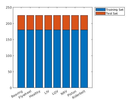
Examine the number of examples in each class. There are 225 recordings in each class for a total of 1800 recordings.
countcats(ads.Labels)
ans = 8×1

   225
   225
   225
   225
   225
   225
   225
   225
Split the data into training and test sets. Use 80% of the data for training and hold out the remaining 20% for testing. Shuffle the data once before splitting.
rng default
ads = shuffle(ads);
[adsTrain,adsTest] = splitEachLabel(ads,0.8,0.2);
Verify that the number of examples in each class is the expected number.
uniqueLabels = unique(adsTrain.Labels);
tblTrain = countEachLabel(adsTrain);
tblTest = countEachLabel(adsTest);
H = bar(uniqueLabels,[tblTrain.Count, tblTest.Count],'stacked');
legend(H,["Training Set","Test Set"],'Location','NorthEastOutside')
Select some random examples from the training set for plotting. Each record has 50,000 samples sampled at 16 kHz.
idx = randperm(numel(adsTrain.Files),8);
Fs = 16e3;
for n = 1:numel(idx)
    x = audioread(adsTrain.Files{idx(n)});
    t = (0:size(x,1)-1)/Fs;
    subplot(4,2,n);
    plot(t,x);
    if n == 7 || n == 8
        xlabel('Seconds');
    end
    title(string(adsTrain.Labels(idx(n))));
end

Wavelet Scattering Network
Construct a wavelet scattering network based on the data characteristics. Set the invariance scale to be 0.5 seconds.
N = 5e4;
Fs = 16e3;
IS = 0.5;
sn = waveletScattering('SignalLength',N,'SamplingFrequency',Fs,...
    'InvarianceScale',0.5);
With these network settings, there are 330 scattering paths and 25 time windows per example. You can see this with the following code.
[~,numpaths] = paths(sn);
Ncfs = numCoefficients(sn);
sum(numpaths)
ans = 330
Ncfs
Ncfs = 25
Note this already represents a 6-fold reduction in the size of the data for each record. We reduced the data size from 50,000 samples to 8250. In this case, we obtain a further reduction by subsampling the time windows by a factor of 6, reducing the size of each example by a factor of 25.
Obtain the wavelet scattering features for the training and test sets. If you have a suitable GPU and Parallel Computing Toolbox, you can set useGPU to true to accelerate the scattering transform. The function helperBatchScatFeatures obtains the scattering transform and subsamples the time windows by a factor of 6.
batchsize = 64;
useGPU = false;
scTrain = [];
while hasdata(adsTrain)
    sc = helperBatchScatFeatures(adsTrain,sn,N,batchsize,useGPU);
    scTrain = cat(3,scTrain,sc);
end
Repeat the process for the held out test set.
scTest = [];
while hasdata(adsTest)
   sc = helperBatchScatFeatures(adsTest,sn,N,batchsize,useGPU);
   scTest = cat(3,scTest,sc);
end
scTest = gather(scTest);
Determine the number of scattering paths and the number of time windows. There are 330 scattering paths and five time windows.
[Npaths,numTimeWindows,~] = size(scTrain);
Reshape the scattering transforms for the training and test sets so that each row is a time window across all 330 scattering paths. Because there are five time windows in this subsampled wavelet scattering transform, the size of TrainFeatures is 5*1440-by-330. Similarly, the size of TestFeatures is 5*360-by-330.
TrainFeatures = permute(scTrain,[2 3 1]);
TrainFeatures = reshape(TrainFeatures,[],Npaths,1);
TestFeatures = permute(scTest,[2 3 1]);
TestFeatures = reshape(TestFeatures,[],Npaths,1);
In order to fit our SVM model, replicate the labels so that there is a label for each row of TrainFeatures.
trainLabels = adsTrain.Labels;
numTrainSignals = numel(trainLabels);
trainLabels = repmat(trainLabels,1,numTimeWindows);
trainLabels = reshape(trainLabels',numTrainSignals*numTimeWindows,1);
SVM Classification
Use a multi-class support vector machine (SVM) classifier with a cubic polynomial kernel. Fit the SVM to the training data.
template = templateSVM(...
    'KernelFunction', 'polynomial', ...
    'PolynomialOrder', 3, ...
    'KernelScale', 'auto', ...
    'BoxConstraint', 1, ...
    'Standardize', true);

classificationSVM = fitcecoc(...
    TrainFeatures, ...
    trainLabels, ...
    'Learners', template, ...
    'Coding', 'onevsall','ClassNames',uniqueLabels);
Determine the cross-validation accuracy of the SVM model using 5-fold cross validation.
partitionedModel = crossval(classificationSVM, 'KFold', 5);
validationAccuracy = (1 - kfoldLoss(partitionedModel))*100
validationAccuracy = single
99.5278
The cross-validation accuracy is over 99% when each time window is separately classified. This performance is excellent, but the actual cross-validation accuracy is actually higher. Because there are five windows per example, we should use all five time windows to assign the class label. There are numerous ways to do this, but here we use a simple majority vote over the five windows. If there is no majority, we assign the class "NoUniqueMode" and consider that a classification error.
Obtain the class predictions from the cross-validation model and examine the accuracy using a simple majority vote.
validationPredictions = kfoldPredict(partitionedModel);
TrainVotes = helperMajorityVote(validationPredictions,adsTrain.Labels,uniqueLabels);
crossvalAccuracy = sum(TrainVotes == adsTrain.Labels)/numel(adsTrain.Labels)*100;
crossvalAccuracy
crossvalAccuracy = 100
The cross-validation accuracy is near 100%. Apply the model to the held-out test set. Use a simple majority vote to assign the class label.
predLabels = predict(classificationSVM,TestFeatures);
[TestVotes,TestCounts] = helperMajorityVote(predLabels,adsTest.Labels,uniqueLabels);
testAccuracy = sum(TestVotes == adsTest.Labels)/numel(adsTest.Labels)*100;
testAccuracy
testAccuracy = 100
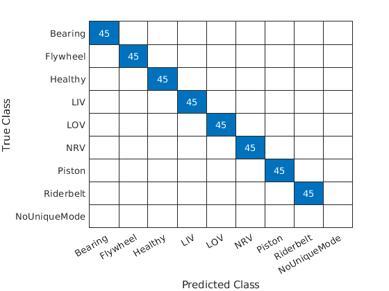
The accuracy on the held-out test set is near 100% indicating that our model generalizes well to unseen data. Plot the confusion chart. Note that each test example produced a majority class (unique mode).
figure
confusionchart(adsTest.Labels,TestVotes)
Summary
In this example, we used the wavelet scattering transform with an SVM to classify faults in an air compressor. The scattering transform provided a robust set of features by which the SVM was able to achieve excellent cross-validation and test performance.
References
[1] Verma, Nishchal K., Rahul Kumar Sevakula, Sonal Dixit, and Al Salour. “Intelligent Condition Based Monitoring Using Acoustic Signals for Air Compressors.” IEEE Transactions on Reliability 65, no. 1 (March 2016): 291–309. https://doi.org/10.1109/TR.2015.2459684.
Supporting Functions
helperBatchScatFeatures - This function returns the wavelet time scattering feature matrix for a given input signal. The scattering features are subsampled by a factor of 6. If useGPU is set to true, the scattering transform is computed on the GPU.
function sc = helperBatchScatFeatures(ds,sn,N,batchsize,useGPU)
% This function is only intended to support examples in the Wavelet
% Toolbox. It may be changed or removed in a future release.

% Read batch of data from audio datastore
batch = helperReadBatch(ds,N,batchsize);
if useGPU
    batch = gpuArray(batch);
end

% Obtain scattering features
S = sn.featureMatrix(batch,'transform','log');
gather(batch);
S = gather(S);

% Subsample the features
sc = S(:,1:6:end,:);
end
helperReadBatch - This function reads batches of a specified size from a datastore and returns the output in single precision. Each column of the output is a separate signal from the datastore. The output may have fewer columns than the batchsize if the datastore does not have enough records.
function batchout = helperReadBatch(ds,N,batchsize)
% This function is only in support of Wavelet Toolbox examples. It may
% change or be removed in a future release.
%
% batchout = readReadBatch(ds,N,batchsize) where ds is the Datastore and
%   ds is the Datastore
%   batchsize is the batchsize

kk = 1;

while(hasdata(ds)) && kk <= batchsize
    tmpRead = read(ds);
    batchout(:,kk) = cast(tmpRead(1:N),'single'); %#ok<AGROW>
    kk = kk+1;
end

end
helperMajorityVote - This function obtains the majority vote for the class labels. If there is no majority, "NoUniqueMode" is returned and treated as an error.
function [ClassVotes,ClassCounts] = helperMajorityVote(predLabels,origLabels,classes)
% This function is in support of wavelet scattering examples only. It may
% change or be removed in a future release.

% Make categorical arrays if the labels are not already categorical
predLabels = categorical(predLabels);
origLabels = categorical(origLabels);
% Expects both predLabels and origLabels to be categorical vectors
Npred = numel(predLabels);
Norig = numel(origLabels);
Nwin = Npred/Norig;
predLabels = reshape(predLabels,Nwin,Norig);
ClassCounts = countcats(predLabels);
[mxcount,idx] = max(ClassCounts);
ClassVotes = classes(idx);
tmpsum = sum(ClassCounts == mxcount);
ClassVotes(tmpsum > 1) = categorical({'NoUniqueMode'});
end