Time-Series Classification Using Complex-Valued Deep Learning

Data Description

This example uses PCG data obtained from persons with normal and abnormal cardiac function. The data set consists of 3829 recordings, 2575 from persons with normal cardiac function and 1254 from persons with abnormal cardiac function. Each recording is 10,000 samples long and is sampled at 2 kHz. This represents five seconds of phonocardiogram data. The data set is constructed from the training and validation data used in the PhysioNet Computing in Cardiology Challenge 2016 [[1],[3].

Download Data

The first step is to download the data from the GitHub repository. To download the data, click Code and select Download ZIP. Save the file physionet_phonocardiogram-main.zip in a folder where you have write permission. The instructions for this example assume you have downloaded the file to your temporary directory, (tempdir in MATLAB®). Modify the subsequent instructions for unzipping and loading the data if you choose to download the data in a folder different from tempdir.

The file physionet_phonocardiogram-main.zip contains

and PCG_Data.zip contains

heartSoundData.mat holds the data and class labels used in this example. The .txt file, Modified_physionet_data.txt, is required by PhysioNet's copying policy and provides the source attributions for the data as well as a description of how each signal in heartSoundData.mat corresponds to a file in the original PhysioNet data. extrafiles.mat also contains source file attributions and is explained in the Modified_physionet_data.txt file. The only file required to run the example is heartSoundData.mat.

Load Data

If you followed the download instructions in the previous section, enter the following commands to unzip the two archive files:

unzip(fullfile(tempdir,"physionet_phonocardiogram-main.zip"),tempdir)
unzip(fullfile(tempdir,"physionet_phonocardiogram-main","PCG_Data.zip"), ...
     fullfile(tempdir,"PCG_Data"))

After you unzip the PCG_Data.zip file, load the data into MATLAB:

load(fullfile(tempdir,"PCG_Data","heartSoundData.mat"))

heartSoundData is a structure array with two fields: Data and Classes. Data is a 10000-by-3829 matrix where each column is an PCG recording. Classes is a 3829-by-1 categorical array of diagnostic labels, one for each column of Data. Because this is a binary classification problem, the classes are "normal" and "abnormal". As previously stated, there are 2575 normal records and 1254 abnormal records. Equivalently, 67.25% of the examples in the data are from persons with normal cardiac function while 32.75% are from persons with abnormal cardiac function. You can verify this by entering:

countlabels(heartSoundData.Classes)

ans = 2×3 table
      normal    2575    67.2499
    abnormal    1254    32.7501

Create Training and Test Sets

Split the data into training and test sets. Allocate 70% of the data for training and the remaining 30% for test.

rng default
idxTrainTest = splitlabels(heartSoundData.Classes,0.7);
trainData = heartSoundData.Data(:,idxTrainTest{1});
testData = heartSoundData.Data(:,idxTrainTest{2});
trainLabels = heartSoundData.Classes(idxTrainTest{1});
testLabels = heartSoundData.Classes(idxTrainTest{2});

You can check the count and percentage of each class in the training and test sets.

trainlabelCounts = countlabels(trainLabels)

trainlabelCounts = 2×3 table
      normal    1802    67.2388
    abnormal     878    32.7612

countlabels(testLabels)

ans = 2×3 table
      normal    773    67.2759
    abnormal    376    32.7241

Note that the training and test sets have been partitioned so that the proportion of "normal" and "abnormal" records in the training and test sets are the same as their proportions in the overall data.

Scattering Spectra

Compute the scattering spectra for the entire training set of 2680 signals.

tsn = waveletScattering(SignalLength=1e4,InvarianceScale=7e3,FilterDownsampling="bandlimited",...
    QualityFactors=[1 1],OptimizePath=true,OversamplingFactor=3,Boundary="reflection");
[scatspectraTrain,cfsTable] = scatteringSpectra(tsn,trainData,InputNormalization="std",...
    IncludeLowpass=true);
scatspectraTest = scatteringSpectra(tsn,testData,InputNormalization="std",...
    IncludeLowpass=true);

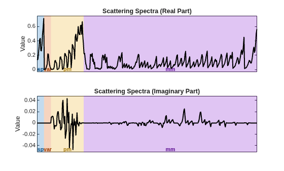
With the given configuration of the scattering network and the scattering spectra computation, each signal yields 377 coefficients. As previously stated, these coefficients are complex-valued in general.

cfsTable is a MATLAB table that provides all the metadata necessary to understand and extract coefficients from the scattering spectra computation. See the documentation for details on how to interpret the coefficients based on the metadata.

The helper function, helperPlotScatteringSpectra, plots the scattering spectra in shaded regions corresponding to the type of coefficient. Plot the real and imaginary parts for the first training example.

tiledlayout(2,1)
nexttile
ax1 = helperPlotScatteringSpectra(real(scatspectraTrain(:,1)),cfsTable.type);
ax1.Title.String ="Scattering Spectra (Real Part)";
nexttile
ax2 = helperPlotScatteringSpectra(imag(scatspectraTrain(:,1)),cfsTable.type);
ax2.Title.String ="Scattering Spectra (Imaginary Part)";

Complex-Valued Deep Learning

Most deep learning networks are explicitly designed for real-valued data. Care must be taken in computing gradients for backpropagation and activation functions when the data are complex-valued. In Deep Learning Toolbox™, a subset of layers, activations, and optimizers support learning on complex-valued data.

Create dlarray tensors suitable for training the network. Since a fully connected network is used, label the dimensions of the tensors as channel-by-batch, "CB".

dlscatspectraTrain = dlarray(scatspectraTrain,"CB");
dlscatspectraTest = dlarray(scatspectraTest,"CB");

Define a network consisting of fully connected layers and ReLU layers which support complex-valued inputs.

layersSS = [
    featureInputLayer(377,Normalization="zscore")    
    complexFullyConnectedLayer(256,Name="complexfc1")
    complexReluLayer(Name="complexrelu1") 
    dropoutLayer(0.6,Name="dropout1")
    complexFullyConnectedLayer(128,Name="complexfc2")
    complexReluLayer(Name="complexrelu2")
    dropoutLayer(0.4,Name="dropout2")
    complexFullyConnectedLayer(32,Name="complexfc3")
    complexReluLayer(Name="complexrelu3")   
    complexFullyConnectedLayer(16,Name="complexfc4")
    complexReluLayer(Name="complexrelu4") 
    complexFullyConnectedLayer(2,Name="complexfc4")
    functionLayer(@abs,Formattable=true,Acceleratable=true)
    softmaxLayer(Name="softmax")
    ];
dlnetSS = dlnetwork(layersSS);

complexFullyConnectedLayer and complexReluLayer are deep learning layers specifically adapted for complex-valued inputs and gradient computation. Since this is a binary classification problem, a cross-entropy loss function is used. This means that we need to convert the output of the network into probabilities. Since the output of complexFullyConnectedLayer(2) is an array of complex numbers 2-by-B, where B is the batch size, we need to convert those complex numbers into real-valued logits prior to calling the softmax operation. In order to do that, simply use a functionLayer which takes the absolute values of 2xB complex-valued matrix immediately preceding softmaxLayer.

Because the data is imbalanced, calculate class weights which are inversely proportional to the class frequencies for use in a weighted cross-entropy loss. Create a customized loss function as a function handle.

datasetSize = size(scatspectraTrain,2);
numClasses = 2;
classWeights = [datasetSize/(numClasses*trainlabelCounts.Count(1)) ...
    datasetSize/(numClasses*trainlabelCounts.Count(2))];
lossFcn = @(Y,T) crossentropy(Y,T,classWeights, ...
    NormalizationFactor="all-elements", ...
    WeightsFormat="C")*numClasses;

Train Complex-Valued fully connected Network

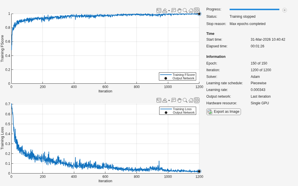
Set up the training options for the network. This small network trains very quickly even when training is done on the CPU. However, if you wish to skip training, you can load a trained network in Scattering Spectra Model Evaluation on Test Set.

The Adam optimizer supports complex-valued data in MATLAB and is used in this example.

optionsSS = trainingOptions("adam", ...
    MaxEpochs=150, ...
    MiniBatchSize=300, ...
    InitialLearnRate=1e-3, ...
    LearnRateSchedule="piecewise", ...
    LearnRateDropFactor=0.7, ...
    LearnRateDropPeriod=40, ...
    L2Regularization=1e-2, ...
    Shuffle="every-epoch", ...
    Plots="training-progress", ... 
    Verbose=false,...
    Metrics="fscore"); 

Train the model for 150 epochs.

netScatteringSpectraPhonocardiogram = trainnet(dlscatspectraTrain,trainLabels,dlnetSS, lossFcn, optionsSS);

Scattering Spectra Model Evaluation on Test Set

Evaluate the model on the held-out test set. If you opted not to train the network in the previous section, a trained model is loaded prior to prediction.

if ~exist("netScatteringSpectraPhonocardiogram","var")
    load(fullfile(pwd,"netScatteringSpectraPhonocardiogram.mat"));
end
scoresScatSpectra = predict(netScatteringSpectraPhonocardiogram,dlscatspectraTest);
predlabelsScatSpectra = scores2label(scoresScatSpectra,categories(testLabels));
accScatSpectra = sum(predlabelsScatSpectra'==testLabels)/numel(testLabels)*100

accScatSpectra = 
91.4708

The accuracy is approximately 91% on repeated training and inference tests. A subsequent section, Precision and Recall Comparison, compares the confusion chart for the two classes along with the recall (true positive rate) and precision (positive predictive value) metrics obtained using deep learning networks with the scattering spectra and raw data.

Comparison with Raw Data

It is important to compare the approach we have followed of first computing features as inputs to a deep learning network with a network that operates on the raw data. Because the raw waveforms contain 10,000 samples each, some care must be exercised in choosing a network architecture. Here we use a convolutional 1-D architecture, which can process time series of this size efficiently and was found to be more robust on this data than a fully connected network and networks using gated recurrent units (GRU) trained on this data. See the appendix for a sample fully connected network which only achieved around 67% on the test data, fully connected Network on Raw Data, and a GRU network which achieved approximately 75%, GRU Network on Raw Data.

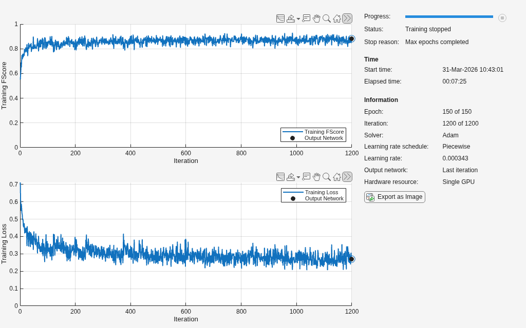
Training the convolutional network requires significantly more time than the network in the previous section. If you wish to skip training, you can load a trained network in the Test Performance on Raw Data.

Obtain "CBT" dlarray tensors for training. The training and test data arrays are in Time-by-Batch format. Specifying the format as "TBC" converts the output dlarray to the canonical "CBT" format for use in convolution1dLayer.

dltrainraw = dlarray(trainData,"TBC");
dltestraw = dlarray(testData,"TBC");

1-D Convolutional Network

Define a 1-D convolutional network.

numChannels = 1;
signalLength = 1e4;
layersConv1d = [    
    sequenceInputLayer(numChannels, Name="input", ...
    MinLength=signalLength,Normalization="zscore")    
    convolution1dLayer(32, 15,Name="conv1")
    batchNormalizationLayer(Name="bn1")
    reluLayer(Name="relu1")
    maxPooling1dLayer(4,Stride=4,Name="pool1")
    convolution1dLayer(9, 64,Name="conv2")
    batchNormalizationLayer(Name="bn2")
    reluLayer(Name="relu2")
    maxPooling1dLayer(4, Stride=4,Name="pool2")
    convolution1dLayer(5, 128,Name="conv3")
    batchNormalizationLayer(Name="bn3")
    reluLayer(Name="relu3")    
    globalAveragePooling1dLayer(Name="gap")   
    fullyConnectedLayer(64,Name="fc1")
    reluLayer(Name="relu4")
    dropoutLayer(0.4, Name="dropout")
    fullyConnectedLayer(2, Name="fc2")
    softmaxLayer(Name="softmax")
    ];
    dlconvnet = dlnetwork(layersConv1d);

Set the training options. The training options are identical to those used in training the fully connected network. The training options are saved in a separate variable to facilitate modification and iteration. Use the same weighted cross-entropy loss.

optionsconv1d = trainingOptions("adam", ...
     MaxEpochs=150, ...
     MiniBatchSize=300, ...
     InitialLearnRate=1e-3, ...
     LearnRateSchedule="piecewise", ...
     LearnRateDropFactor=0.7, ...
     LearnRateDropPeriod=40, ...
     L2Regularization=1e-2, ...
     Shuffle="every-epoch", ...
     Verbose=false, ...
     Plots="training-progress", ...
     Metrics="fscore");
netconv1dPhonocardiogramRawData = trainnet(dltrainraw,trainLabels,dlconvnet,lossFcn, optionsconv1d);

Test Performance on Raw Data

Test the trained convolutional network on the raw data. If you opted not to train the network in the previous section, a trained model is loaded prior to prediction.

if ~exist("netconv1dPhonocardiogramRawData","var")
    load netconv1dPhonocardiogramRawData.mat
end
scoresConv = minibatchpredict(netconv1dPhonocardiogramRawData,dltestraw);
predLabelsConv = scores2label(scoresConv,categories(testLabels));
accuracyConv = sum(predLabelsConv'==testLabels)/numel(testLabels)*100

accuracyConv = 
89.8172

The accuracy on the raw data is also quite good at approximately 89%. However, it requires significantly longer to train the network with the raw data due to the dimensionality of the raw data as compared with the length of scattering spectra.

Precision and Recall Comparison

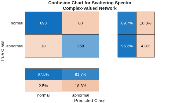
Compare the performance of the scattering spectra (complex-valued) network against the raw data in terms of precision and recall. Plot the confusion charts for both the scattering spectra and raw data predictions.

figure
cchartScatSpectra= confusionchart(testLabels,predlabelsScatSpectra,...
    ColumnSummary="column-normalized",RowSummary="row-normalized");
title(["Confusion Chart for Scattering Spectra" ;"Complex-Valued Network"])

figure
cchartRawData = confusionchart(testLabels,predLabelsConv ,...
    ColumnSummary="column-normalized",RowSummary="row-normalized");
title("Confusion Chart for Raw Data")

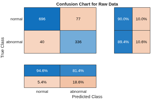
Summarize the precision, recall, F1, and macro-averaged scores for the scattering spectra using the helperF1heartSounds helper function.

PRTableSS = helperF1heartSounds(cchartScatSpectra.NormalizedValues);
fprintf("Scattering Spectra")

Scattering Spectra

disp(PRTableSS)

                     Precision    Recall    F1_Score
                     _________    ______    ________

    Abnormal          81.735      95.213     87.961 
    Normal            97.468      89.651     93.396 
    Macro Average     89.602      92.432     90.678 

Do the same for the raw data.

PRTableRaw = helperF1heartSounds(cchartRawData.NormalizedValues);
fprintf("Raw Data")

Raw Data

disp(PRTableRaw)

                     Precision    Recall    F1_Score
                     _________    ______    ________

    Abnormal          81.356      89.362     85.171 
    Normal            94.565      90.039     92.247 
    Macro Average     87.961        89.7     88.709 

The macro-averaged metrics for the scattering spectra network are quite good and superior to the network trained on the raw data. However, in repeated testing, the performance of the networks was actually quite similar. Due to the stochastic nature of deep learning, you may find different results upon retraining these networks even without modifying hyperparameters.

Summary

In this example, two deep networks were trained to discriminate between phonocardiogram recordings indicative of normal and abnormal cardiac function. One network was trained on the complex-valued scattering spectra coefficients while another network was trained on the raw data. In this example, the network performances were comparable but the reduced dimensionality of the scattering spectra features makes that network significantly faster to train. That is an advantage because it permits faster iteration with different hyperparameter settings.

There are many modifications that can be made in each case to change the performance metrics. The innovation in this example is the use of a complex-valued neural network. These networks make gradient-descent based learning on complex-valued data with high accuracy possible.

References

Appendix

Supporting Functions

function PRTable = helperF1heartSounds(confmat)
% This function is only in support of Scattering Spectra and 
% Wavelet Phase Harmonics with Phonocardiogram Data It may change or be
% removed in a future release.

% Copyright 2026 The MathWorks, Inc. 
precisionAB = confmat(2,2)/sum(confmat(:,2))*100;
precisionNR = confmat(1,1)/sum(confmat(:,1))*100 ;
recallAB = confmat(2,2)/sum(confmat(2,:))*100;
recallNR = confmat(1,1)/sum(confmat(1,:))*100;
F1AB = 2*(precisionAB*recallAB)/(precisionAB+recallAB);
F1NR = 2*(precisionNR*recallNR)/(precisionNR+recallNR);
MacroAverages = mean(cat(2,[precisionAB; precisionNR],...
    [recallAB; recallNR], [F1AB ; F1NR]));
% Construct a MATLAB Table to display the results.
PRTable = array2table([precisionAB recallAB F1AB;...
    precisionNR recallNR F1NR; ...
    MacroAverages],...
    VariableNames = ["Precision","Recall","F1_Score"],...
    RowNames = ["Abnormal","Normal","Macro Average"]);
end

function ax = helperPlotScatteringSpectra(cfs,cfstype)
% This function is for use in MathWorks' examples only. It may change or be
% removed in a future release.

% Copyright 2026 The MathWorks, Inc.
% ── Plot parameters ─────────────────────────────────────────────────────────────
alpha_val = 0.25;
line_width = 1.5;
line_color = 'k';
% Check that the number of coefficients matches the number of categories.
assert(numel(cfs) == numel(cfstype), ...
    'CFS and CFSTYPE must have the same number of elements.');
% ── Derive block boundaries ───────────────────────────────────────────────────
[uCats, blockStarts] = unique(cfstype, 'stable');
blockEnds   = [blockStarts(2:end) - 1; numel(cfs)];
blockCenters = (blockStarts + blockEnds) / 2;
colorOrder = get(groot, 'DefaultAxesColorOrder');
% ── Plot ──────────────────────────────────────────────────────────────────────
ax = newplot;
hold(ax, 'on');
yLimPad = 0.05 * (max(cfs) - min(cfs));
yLo = min(cfs) - yLimPad;
yHi = max(cfs) + yLimPad;
for k = 1:numel(uCats)
    xs  = blockStarts(k) - 0.5;
    xe  = blockEnds(k)   + 0.5;
    col = colorOrder(mod(k-1, size(colorOrder,1)) + 1, :);
    patch(ax, [xs xe xe xs], [yLo yLo yHi yHi], col, ...
        'FaceAlpha',alpha_val, ...
        'EdgeColor', 'none', ...
        'HandleVisibility', 'off');
    text(ax, blockCenters(k), yLo, char(uCats(k)), ...
        'HorizontalAlignment', 'center', ...
        'VerticalAlignment',   'bottom', ...
        'FontWeight',          'bold', ...
        'Color',               col*0.7,...
        'FontSize',8);   % darker shade of patch color
end
plot(ax, 1:numel(cfs), cfs(:)', ...
    'Color', line_color, ...
    'LineWidth', line_width, ...
    'HandleVisibility', 'off');
% ── Formatting ────────────────────────────────────────────────────────────────
ylim(ax, [yLo yHi]);
xlim(ax, [0.5, numel(cfs) + 0.5]);
set(ax, 'XTick', []);
ylabel(ax, 'Value');
box(ax, 'on');
hold(ax, 'off');
end

Fully Connected Network on Raw Data

The following fully connected network was trained and evaluated on the raw data. This network only achieved about 67% accuracy on the test set.

layersFCRaw = [
    featureInputLayer(1e4)
    fullyConnectedLayer(512,Name="fc1")
    batchNormalizationLayer(Name="bn1")
    reluLayer(Name="relu1")
    dropoutLayer(0.4,Name="drop1")   
    fullyConnectedLayer(256, Name="fc2")
    batchNormalizationLayer(Name="bn2")
    reluLayer(Name="relu2")
    dropoutLayer(0.4, Name="drop2")    
    fullyConnectedLayer(128, Name="fc3")
    batchNormalizationLayer(Name="bn3")
    reluLayer(Name="relu3")
    dropoutLayer(0.3, Name="drop3")    
    fullyConnectedLayer(64, Name="fc4")
    batchNormalizationLayer(Name="bn4")
    reluLayer(Name="relu4")
    dropoutLayer(0.3,Name="drop4")    
    fullyConnectedLayer(2, Name="fc_out")
    softmaxLayer(Name="softmax")
    ];

GRU Network on Raw Data

The following GRU network was trained and evaluated on the raw data. One version uses numFeatures=1 and inputs the entire raw time series as one segment. Another model was trained and evaluated by setting numFeatures=5 and reshaping the data into a 2000-by-5-by-Batch tensor. This GRU network trained on the entire time series achieved around 75% accuracy, while the network trained on segmenting the data into 5 segments achieved approximately 63% on test.

numHiddenUnits1 = 64;
numHiddenUnits2 = 32;
numClasses      = 2;
dropoutRate      = 0.3;
numFeatures = 1;
layersGRU = [
    sequenceInputLayer(numFeatures, Name="input")
    gruLayer(numHiddenUnits1, ...
    OutputMode="sequence", ...
    Name="gru1")
    dropoutLayer(dropoutRate, 'Name', 'drop1')
    % Output the final hidden state
    gruLayer(numHiddenUnits2, ...
    OutputMode="last", ...       
    Name="gru2")
    dropoutLayer(dropoutRate, Name="drop2")
    fullyConnectedLayer(numClasses, Name="fc")
    softmaxLayer(Name="softmax")    
    ];

References

Goldberger, A. L., L. A. N. Amaral, L. Glass, J. M. Hausdorff, P. Ch. Ivanov, R. G. Mark, J. E. Mietus, G. B. Moody, C.-K. Peng, and H. E. Stanley. "PhysioBank, PhysioToolkit, and PhysioNet: Components of a New Research Resource for Complex Physiologic Signals". Circulation. Vol. 101, No. 23, 13 June 2000, pp. e215-e220. https://circ.ahajournals.org/content/101/23/e215.full.
Lempereur, Etienne, Nathanaël Cuvelle–Magar, Florentin Coeurdoux, Stéphane Mallat, and Eric Vanden-Eijnden. 2026. "MGD: Moment Guided Diffusion for Maximum Entropy Generation." arXiv preprint. https://arxiv.org/abs/2602.17211.
Liu et al. "An open access database for the evaluation of heart sound algorithms". Physiological Measurement. Vol. 37, No. 12, 21 November 2016, pp. 2181-2213. https://www.ncbi.nlm.nih.gov/pubmed/27869105.
Mallat, Stephane, Sixin Zhang, and Gaspar Rochette. 2019. "Phase harmonic Correlations and Convolutional Neural Networks". Journal of Information and Inference, 721-747, https://doi.org/10.1093/imaiai/iaz019.
Morel, Rudy, Gaspar Rochette, Roberto Leonarduzzi, Jean-Philippe Bouchaud, and Stéphane Mallat. 2024. "Scale Dependencies and Self-Similar Models with Wavelet Scattering Spectra." Applied and Computational Harmonic Analysis, November, 101724–24. https://doi.org/10.1016/j.acha.2024.101724.
Regaldo-Saint Blanchard, Bruno, Erwan Allys, Constant AuClair, Francois Boulanger, Michael Eickenburg, Francois Levrier, Leo Vacher, and Sixin Zhang. 2023. "Generative Models of Multi-channel Data from a Single Example - Application to Dust Emission." The Astrophysical Journal 943 (2023): 9. https://doi.org/10.3847/1538-4357/aca538.