Wavelet Scattering Spectra
R2026bWavelet scattering spectra provide a method to capture correlations in data across time and scales. The technique uses a wavelet time scattering network to derive summary statistics that measure correlations across scales. (To learn more about wavelet scattering, see Wavelet Scattering.) You can use the statistics as features in machine learning and AI workflows. The examples Scattering Spectra and Wavelet Phase Harmonics with Phonocardiogram Data and Time-Series Classification Using Complex-Valued Deep Learning illustrate two such workflows.
A strength of wavelet-based techniques is their proven utility in analyzing multi-scale non-Gaussian processes with at least stationary increments. Because the wavelet transform separates variations in time series across multiple scales, you can use the transform to analyze correlations across scales. Morel, Rochette, Leonarduzzi, Bouchaud, and Mallat introduced wavelet scattering spectra [7]. Leveraging the wavelet scattering transform, they showed how to use joint correlation of wavelet coefficients and their modulus to identify dependencies across scales. The scattering spectra consist of five sets of coefficients of different types. Each type is sensitive to a different property of the random process.
Wavelet sparsity factors
Variance (wavelet spectrum)
Phase-modulus cross spectrum
Modulus-modulus correlations (scattering cross-spectrum)
Wavelet phase harmonics
Motivation
For a wavelet and dilation parameter λ > 0,
where the bar denotes the complex conjugate. Using this convention, the wavelet transform of x at scale λ as a convolution is:
If you try to compare wavelet coefficients from different scales, their correlation will be essentially zero if the wavelets are sufficiently separated in scale. You can demonstrate this using Parseval's theorem:
For λ and λ' sufficiently separated, . If λ = λ',
Evaluating the above expression across different values of λ yields a collection known as the wavelet power
spectrum. You can use the cwtfilterbank
object function timeSpectrum
to obtain the time-averaged wavelet power spectrum.
Wavelet Scattering Spectra
For details and the theoretical development of wavelet scattering spectra, see [7].
In the discussion that follows, denotes a wavelet in the first filter bank and denotes a wavelet in the second filter bank.
Wavelet Sparsity Factors
The wavelet sparsity factors are the ratios of the first and second moments of the first-order wavelet scalogram coefficients. The wavelet sparsity factors are defined as:
where N is the number of wavelet coefficients, k is the wavelet filter index in the first filter bank, and is the biased standard deviation of the wavelet coefficients.
By default, the scatteringSpectra function returns sparsity factors that include a term
for the lowpass filter φ(t):
where σφ is the root mean square (RMS) instead of the standard deviation. Because the scaling function is real-valued, the absolute value is not necessary.
By using the RMS, the scatteringSpectra function protects against edge cases where the sparsity
coefficient corresponding to the lowpass filter would otherwise blow up in value.
Consider the following equality:
where μ is the mean and is the biased estimate of the standard deviation:
Because the mean of the wavelet coefficients is zero, the RMS and the biased standard deviation are equal. However, for φ(t), the scaling function, the situation is different. For the constant signal, the standard deviation is zero but the mean is equal to the value of each element in the signal. Therefore, the denominator σφ is not zero.
Variance (Wavelet Spectrum)
The variance, or wavelet spectrum, is defined as:
These features tend to differentiate signals with differing long-range dependencies. By default, there is an additional term corresponding to the lowpass filter:
Phase-Modulus Cross Spectrum
The phase-modulus cross spectrum is the correlation between the wavelet coefficients and their modulus:
where the filter indices satisfy l > k. Morel et al. [7] show that taking the modulus enables you to obtain some correlation with wavelet coefficients at a different scale. The power spectrum of overlaps the power spectrum of .
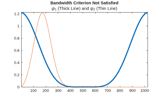
As implemented, for a given , the scatteringSpectra function chooses those wavelets such that 1/2 the 3-dB bandwidth of overlaps the center frequency of minus 1/2 its 3-dB bandwidth. For more information, see Visualize Wavelet Filter Bandwidth Criterion.
The phase-modulus coefficients tend to differentiate signals based on their skewness. In other words, the phase modulus is sensitive to time asymmetries in the signal. Note that the coefficients involve only wavelets from the first filter bank, which can potentially contain more wavelets than the second filter bank.
Modulus-Modulus Correlation (Scattering Cross-Spectrum)
The modulus-modulus correlations, or scattering cross-spectrum, are defined as
where the filter indices satisfy k ≥ k', l − k ≠ 0, and l − k' ≠ 0. The scattering cross-spectrum depends on the wavelet filters in the first and second filter banks. These coefficients quantify envelope dependencies across scales because they capture correlations between the envelopes of the wavelet coefficients, .
The scatteringSpectra function applies a bandwidth criterion similar to the
one used for the phase-modulus cross spectrum. However, in this case, the criterion
involves filters in the first and second filter banks. For a filter , the function chooses those filters such that 1/2 the 3-dB bandwidth of overlaps the center frequency of minus 1/2 its 3-dB bandwidth.
Similar to the situation with the phase-modulus cross spectrum, wavelet filter indices must satisfy l > k and l > k' when adjusted for the possibility of different quality factors. For example, suppose both filter banks in the wavelet time scattering network have the same Q factor. Then
is valid but scatteringSpectra does not return its conjugate (Hermitian adjoint term).
The function also only pairs lowpass filters with lowpass filters: For more information, see Network Quality Factors and Scattering Spectra.
Wavelet Phase Harmonics
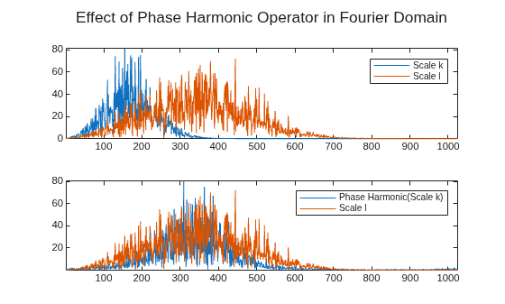
Other strategies for correlating wavelet coefficients at different scales involve using nonlinear transformations to overcome the issue whereby wavelets at different scales might have non-overlapping spectra. One such approach is to compute the wavelet phase harmonics. For a complex number , the phase harmonics are computed as , where is the phase angle of and is a positive integer. Note that the phase harmonics operator does not alter the modulus.
Computing wavelet phase harmonics amounts to a nonlinear dilation in the Fourier domain without affecting the temporal (or spatial) localization of the wavelet. See [5] for the theoretical development of wavelet phase harmonics and [1], [9], and [12] to see wavelet phase harmonics applied to data.
Demonstrate how the phase harmonic operator can align phases for wavelet coefficients at different scales. For reproducibility, initialize the random seed to the default value. Create a random signal with 1024 samples. Create a wavelet scattering network appropriate for the signal. Each network filter bank has a quality factor of 1. In order to obtain the scattering spectra, set the filter downsampling criterion to "bandlimited".
rng("default")
sig = randn(1024,1);
tsn = waveletScattering(QualityFactors=[1 1], ...
    FilterDownsampling="bandlimited");
Use the scatteringSpectra object function to obtain the metadata associated with the scattering spectra of the signal. To obtain metadata associated with the phase harmonics, set the scattering spectra method to "phaseharmonic".
[~,metadataTable] = scatteringSpectra(tsn,sig,Method="phaseharmonic");Use the filterbank object function to obtain the network filter banks. Extract the wavelet filters from the first filter bank.
psif = filterbank(tsn);
psift = psif{2}.psift;
The wavelet filters are defined in the Fourier domain. Use the filters to obtain the wavelet transform of the signal.
wavcfs = ifft(fft(sig).*psift);
In the scattering spectra, the wavelet phase harmonic coefficients are defined as , where is the signal, is the order of the harmonic, and and are the RMS of the wavelet coefficients at scales and , respectively.
From the scattering spectra metadata table, extract the metadata associated with the phase harmonic coefficients. Extract the table variables jl1, jr1, and harmonic. The variables correspond to , , and , respectively, in the inner product.
ind = ismember(metadataTable.type,"ph");
phTable = metadataTable(ind,["jl1" "jr1" "harmonic"])
phTable = 25×3 table
    jl1    jr1    harmonic
    ___    ___    ________

     2      1        2
     3      2        2
     4      3        2
     5      4        2
     6      5        2
     7      6        2
     3      1        3
     4      2        3
     5      3        3
     6      4        3
     7      5        3
     3      1        4
     4      2        4
     5      3        4
     6      4        4
     7      5        4
      ⋮
Choose a row. Obtain the wavelet coefficients and , where equals jl1 and equals jr1.
row = 1;
k = phTable.jl1(row);
l = phTable.jr1(row);

wavA = wavcfs(:,k);
wavB = wavcfs(:,l);
Let p equal the harmonic value of the chosen row. Determine the phase angles of the coefficients . Then apply the phase harmonic operator of order to those coefficients.
p = phTable.harmonic(row);
theta = atan2(imag(wavA),real(wavA));
wavAph = abs(wavA).*exp(1i*theta*p);
Show how applying the phase harmonic operator affects the scale wavelet coefficients in the Fourier domain. Compare the magnitudes of the Fourier transforms of and . Then compare the magnitudes of the Fourier transforms of and . The phase harmonic operator increases the overlap of the spectra of the level and coefficients without affecting the temporal localization of the wavelet.
t=tiledlayout(2,1);
nexttile
plot([abs(fft(wavA)) abs(fft(wavB))])
axis tight
legend("Scale k","Scale l")
nexttile
plot([abs(fft(wavAph)) abs(fft(wavB))])
axis tight
legend("Phase Harmonic(Scale k)","Scale l")
title(t,"Effect of Phase Harmonic Operator in Fourier Domain")
Network Quality Factors and Scattering Spectra
Because the modulus-modulus coefficients depend on the wavelet filters in the first and
second filter banks, specifying too large a filter bank quality factor can easily result in
obtaining more modulus-modulus coefficients than sample points in the original signal. If
you want to avoid this situation, you can either specify smaller quality factors when
creating the scattering network or use scatteringSpectra to compute the wavelet phase harmonics instead of the
modulus-modulus coefficients.
To replace the modulus-modulus coefficients with the wavelet phase harmonics in the
output of scatteringSpectra, set the Method name-value argument
to "phaseharmonic". When you specify that method, for each wavelet
filter , the function finds all other wavelets such that the p
phase harmonic overlaps in frequency. The function does this for phase harmonics p = 2, …, J, where J is essentially the number of octaves that
matches the network invariance scale.
In general, replacing the modulus-modulus coefficients with the wavelet phase harmonics results in a significant reduction of scattering spectra, particularly when the quality factor of the first filter bank is greater than 1. For more information, see the example Compare Coefficient Counts for Different Quality Factors and Methods.
Visualize Wavelet Filter Bandwidth Criterion
You can use the waveletScattering object function filterbank to visualize the bandwidth criterion that the scatteringSpectra function applies to wavelet filters.
Create a wavelet scattering network.
tsn = waveletScattering(FilterDownsampling="bandlimited",QualityFactors=[1,1]);Use the filterbank function to obtain the wavelet filters and their metadata. The filters are in descending order, based on center frequency.
[FBFilters,~,fparams] = filterbank(tsn);
For every wavelet filter in the network, the metadata contains the wavelet center frequency and 3-dB bandwidth . Consider the filters in the first filter bank. Choose the first wavelet filter, . Use the metadata to create a logical array that identifies which filters satisfy the bandwidth criterion .
overlappedPsi = fparams{2}.omegapsi-fparams{2}.psi3dBbw/2 < ...
    fparams{2}.psi3dBbw(1)/2
overlappedPsi = 1×7 logical array
0 0 1 1 1 1 1
Obtain the filter . Plot the Fourier transform of its magnitude. Compare with the wavelet filters that satisfy the criterion.
psif = FBFilters{2}.psift;
psi1abs = abs(ifftshift(ifft(psif(:,1))));
psiabsf = fft(psi1abs);
plot(abs(psiabsf),LineWidth=3)
hold on
plot(psif(:,overlappedPsi))
hold off
axis tight
title("Bandwidth Criterion Satisfied", ...
    "\psi_1 (Thick Line) and \psi_k (Thin Lines)")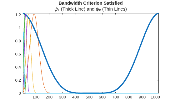
The second wavelet filter, , does not satisfy the criterion. Compare the Fourier transform of with .
plot(abs(psiabsf),LineWidth=3)
hold on
plot(psif(:,2))
hold off
axis tight
title("Bandwidth Criterion Not Satisfied","\psi_1 (Thick Line) and \psi_2 (Thin Line)")
References
[1] Allys, E., T. Marchand, J. F. Cardoso, F. Villaescusa-Navarro, S. Ho, and S. Mallat. “New Interpretable Statistics for Large-Scale Structure Analysis and Generation.” Physical Review D 102, no. 10 (2020): 103506. https://doi.org/10.1103/PhysRevD.102.103506.
[2] Cheng, Sihao, Rudy Morel, Erwan Allys, Brice Ménard, and Stéphane Mallat. “Scattering Spectra Models for Physics.” PNAS Nexus 3, no. 4 (2024): pgae103. https://doi.org/10.1093/pnasnexus/pgae103.
[3] Führ, Hartmut, and Max Getter. “Energy Propagation in Scattering Convolution Networks Can Be Arbitrarily Slow.” Applied and Computational Harmonic Analysis 79 (October 2025): 101790. https://doi.org/10.1016/j.acha.2025.101790.
[4] Mallat, Stéphane. “Group Invariant Scattering.” Communications on Pure and Applied Mathematics 65, no. 10 (October 2012): 1331–98. https://doi.org/10.1002/cpa.21413.
[5] Mallat, Stéphane, Sixin Zhang, and Gaspar Rochette. “Phase Harmonic Correlations and Convolutional Neural Networks.” Information and Inference: A Journal of the IMA 9, no. 3 (2020): 721–47. https://doi.org/10.1093/imaiai/iaz019.
[6] Lei, Minjie, S. E. Clark, Rudy Morel, et al. “Neutral Gas Phase Distribution from HI Morphology: Phase Separation with Scattering Spectra and Variational Autoencoders.” Preprint, arXiv, 2025. https://doi.org/10.48550/ARXIV.2505.20407.
[7] Morel, Rudy, Gaspar Rochette, Roberto Leonarduzzi, Jean-Philippe Bouchaud, and Stéphane Mallat. “Scale Dependencies and Self-Similar Models with Wavelet Scattering Spectra.” Applied and Computational Harmonic Analysis 75 (February 2025): 101724. https://doi.org/10.1016/j.acha.2024.101724.
[8] Morel, Rudy, Stéphane Mallat, and Jean-Philippe Bouchaud. “Path Shadowing Monte-Carlo.” Preprint, arXiv, 2023. https://doi.org/10.48550/ARXIV.2308.01486.
[9] Régaldo-Saint Blancard, Bruno, Erwan Allys, Constant Auclair, et al. “Generative Models of Multichannel Data from a Single Example—Application to Dust Emission.” The Astrophysical Journal 943, no. 1 (2023): 9. https://doi.org/10.3847/1538-4357/aca538.
[10] Siahkoohi, Ali, Rudy Morel, Randall Balestriero, et al. “Multi-Scale Clustering and Source Separation of InSight Mission Seismic Data.” Preprint, arXiv, 2023. https://doi.org/10.48550/ARXIV.2305.16189.
[11] Portilla, Javier, and Eero P. Simoncelli. “A Parametric Texture Model Based on Joint Statistics of Complex Wavelet Coefficients.” International Journal of Computer Vision 40, no. 1 (2000): 49–70. https://doi.org/10.1023/A:1026553619983.
[12] Zhang, Sixin, and Stéphane Mallat. “Maximum Entropy Models from Phase Harmonic Covariances.” Applied and Computational Harmonic Analysis 53 (July 2021): 199–230. https://doi.org/10.1016/j.acha.2021.01.003.
[13] Pipiras, Vladas, and Murad S. Taqqu. Long-Range Dependence and Self-Similarity. Cambridge Series in Statistical and Probabilistic Mathematics 45. Cambridge University Press, 2017.

