Creating Specialized Charts with MATLAB Object-Oriented Programming
By Ken Deeley and David Sampson, MathWorks
Developing advanced MATLAB® visualizations often involves managing multiple low-level graphics objects. This is especially the case for applications containing graphics that update dynamically. Such applications may require time-consuming programming.
A chart object provides a high-level application programming interface (API) for creating custom visualizations. A chart not only provides a convenient visualization API for your end users; it also removes the need for the user to implement low-level graphics programming.
MATLAB includes an object-oriented framework for developing custom charts via the following container superclasses:
matlab.graphics.chartcontainer.ChartContainer(introduced in R2019b)matlab.ui.componentcontainer.ComponentContainer(introduced in R2020b)
This article provides a step-by-step guide, with design patterns and best practices, to creating and implementing a custom chart using this framework. The steps are illustrated with an example scatter plot containing the best-fit line. Topics include:
- Writing a standard chart template
- Writing the chart’s
setupandupdatemethods - Encapsulating data and graphics
- Providing a high-level API for end users
- Including interactive controls
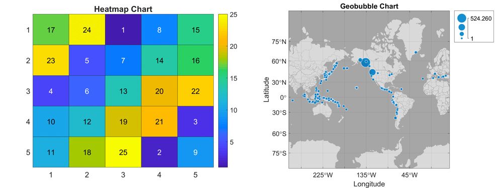
Figure 1. The heatmap and geobubble charts.
In addition, we've created several application-specific charts (Figure 2). You can download these charts, together with the MATLAB code used in this article, from File Exchange.
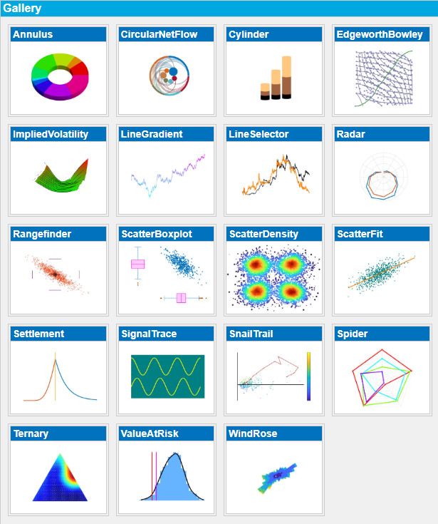
Figure 2. Custom charts available for download on File Exchange.
Creating a 2D Scatter Plot
Let's say we want to create a 2D scatter plot containing the corresponding line of best fit (Figure 3). We could use the scatter function to visualize the discrete (x,y) data points and the fitlm function from Statistics and Machine Learning Toolbox™ to compute the best-fit line.
rng("default")
x = randn(1000, 1);
y = 2*x + 1 + randn(size(x));
s = scatter(x, y, 6, "filled", "MarkerFaceAlpha", 0.5);
m = fitlm(x, y);
hold on
plot(x, m.Fitted, "LineWidth", 2)

Figure 3. Best-fit line and the underlying scattered data.
The code above is sufficient for static visualizations. However, if the application requires the data to be dynamically modifiable, then we encounter several challenges:
- If we replace the
XDataorYDatawith a new array of the same length as the currentXData, the best-fit line is not dynamically updated (Figure 4).s.XData = s.XData + 4;
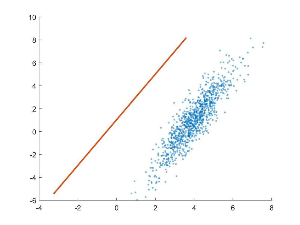
Figure 4. The best-fit line is not updated after changing the XData of the scatter plot.
- The
Scatterobjectsissues a warning, and performs no graphics update, if either of its data properties (XDataorYData) is set to an array that is longer or shorter than the current array.s.XData = s.XData(1:500);
We can resolve these challenges, and others, by designing a chart, which we name ScatterFit.
Structuring the Chart Code: Function or Class?
A function encapsulates the code as a reusable unit and lets you create multiple charts without duplicating the code.
function scatterfit(varargin)

% Ensure 2 or 3 inputs.
narginchk(2, 3)

% We support the calling syntax scatterfit(x, y) or
% scatterfit(f, x, y), where f is the parent graphics.
switch nargin
    case 2
        f = gcf;
        x = varargin{1};
        y = varargin{2};
    otherwise % case 3
        f = varargin{1};
        x = varargin{2};
        y = varargin{3};
end % switch/case

% Create the chart axes and scatter plot.
ax = axes("Parent", f);
scatter(ax, x, y, 6, "filled")
% Compute and create the best-fit line.
m = fitlm(x, y);
hold(ax, "on")
plot(ax, x, m.Fitted, "LineWidth", 2)
hold(ax, "off")

end % scatterfit function
Note that this function requires the two data inputs (x and y). You can specify the graphics parent f (for example, a figure) as the first input argument.
scatterfit(x, y)specifies the two data inputs.scatterfit(f, x, y)specifies the graphics parent and the data.
In the first case, the function exhibits autoparenting behavior — that is, a figure for the chart will be created automatically.
Using a function to create a chart has some drawbacks:
- You cannot modify the data after the chart has been created.
- To change the chart data, you need to call the function again to recreate the chart.
- It's difficult for the end user to locate configurable chart parameters (e.g., labels and decorative graphics properties such as color, line style, etc).
Implementing the chart as a class has all the benefits of code encapsulation and reusability that the function provides while also letting you modify the chart without needing to recreate it.
Choosing the Chart Superclass: ChartContainer or ComponentContainer?
A chart must be implemented as a handle class so that it can be modified in place. For consistency with MATLAB graphics objects, charts should support the get/set syntax for properties in addition to the standard dot notation. Both ChartContainer and ComponentContainer are handle classes and provide support for the get/set syntax, which means that you can derive your custom chart from one of these superclasses.
classdef ScatterFit < matlab.ui.componentcontainer.ComponentContainer
As a result, for any property, the syntax shown in Table 1 is automatically supported.
| Syntax Type | Access | Modification |
|---|---|---|
| Dot notation | x = SF.XData; |
SF.XData = x; |
get/set |
x = get(SF, "XData"); |
set(SF, "XData", x) |
Table 1. Access and modification syntax for chart properties.
Select a superclass based on the requirements of your chart. If the chart does not require interactive user-facing controls such as buttons, dropdown menus, and checkboxes, then derive the chart from ChartContainer; otherwise, use ComponentContainer. This is because the chart container superclass provides a tiled layout as the top-level graphics object, and this object can contain axes but not user controls. The top-level graphics object associated with a component container is a panel-like object, which supports both axes and user controls.
Note that the framework superclasses automatically manage the chart life cycle, guaranteeing the following behavior:
- When the chart graphics are deleted (for example, by closing the main figure window), the chart object is deleted.
- When the chart object is deleted (for example, when it goes out of scope or when its handle is deleted), the chart graphics are deleted.
The framework superclasses support the use of name-value pairs for all chart input arguments. This means that no input arguments need to be specified when creating a chart, and all inputs are optional.
Writing the Chart setup and update Methods
We now need to implement two special methods, both of which are required by the framework superclasses:
setup: called automatically when the chart is createdupdate: called automatically when the user modifies certain chart properties
These methods must have protected access in our chart class since they have this attribute in the superclass.
methods (Access = protected)

    function setup(obj)

    end % setup

    function update(obj)

    end % update

end % methods (Access = protected)
Let’s look at the setup method. This is the function within the class definition where we initialize the chart. A good place to start is to copy the code from the scatterfit function to the setup method. We then make the following modifications to support the required chart behavior:
Parent graphics. Unlike the approach described above in the
scatterfitfunction, if noParentinput is specified, then we do not automatically create one for the chart. Note that this behavior is different from that of convenience functions such asplotandscatter, which exhibit autoparenting. Within thesetupmethod, we create our main graphics object (such as an axes, panel, or layout) and assign its parent property to the top-level graphics object provided by the superclass. ThegetLayoutmethod of theChartContainersuperclass returns a reference to the top-level tiled layout. ForComponentContainercharts, we can simply assign the graphics parent property to the object itself.obj.Axes = axes("Parent", obj.getLayout()); % ChartContainer obj.Axes = axes("Parent", obj); % ComponentContainerIf
Parentis specified as an input argument, then it will be set automatically by the superclass, together with any other name-value pairs supplied during chart creation. The superclass will assign the user-specified parent as the parent of the top-level graphics object.Chart graphics. We create and store any graphics objects required by the chart. Most charts will require an axes object together with some axes contents such as line or patch objects. In the
ScatterFitchart, we need aScatterobject and aLineobject.obj.ScatterSeries = scatter(obj.Axes, NaN, NaN); obj.BestFitLine = line(obj.Axes, NaN, NaN);
Note that we initialize these graphics with their data properties set to
NaN. If the user has specified theXDataand/orYDataon construction, then we defer updating the scatter plot and best-fit line to the correspondingsetmethods (discussed later). This coding practice ensures that any errors caused by the user when specifying the name-value pairs will be caught and handled separately.Graphics configuration. We configure the chart graphics by setting any required properties. For example, we may create annotations such as labels or titles, set a specific view of an axes, add a grid, or adjust the color, style or width of a line.
Whenever practical, we use primitive objects (Table 2) to create the chart graphics, because high-level convenience functions reset many existing axes properties when called. However, there are exceptions to this principle: within ScatterFit, we use the non-primitive function scatter to create the graphics object as it supports subsequent changes to individual marker sizes and colors (whereas a single line object does not).
| Primitive Graphics Function | High-Level Graphics Function |
|---|---|
line |
plot |
surface |
surf |
patch |
fill |
Table 2. Examples of primitive and high-level graphics functions.
We’ll return to the chart’s update method later.
Encapsulating Chart Data and Graphics
In most charts, the underlying graphics comprise at least one axes object together with their contents (for example, line or surface objects) or axes peer objects (for example, legends or colorbars). The chart also maintains internal data properties to ensure that the public properties are presented correctly to the end user. We store the underlying graphics and internal data as private chart properties. For example, the ScatterFit chart maintains the following private properties.
properties (Access = private)
        % Internal storage for the XData property.
        XData_ = double.empty(0, 1)
        % Internal storage for the YData property.
        YData_ = double.empty(0, 1)
        % Logical scalar specifying whether a computation is required.
        ComputationRequired = false()
end % properties (Access = private)
We use the naming convention XData_ to indicate that this is the private, internal version of the chart data. The corresponding public data property visible to the user will be named XData.
properties (Access = private, Transient, NonCopyable)
        % Chart axes.
        Axes(1, 1) matlab.graphics.axis.Axes
        % Scatter series for the (x, y) data.
        ScatterSeries(1, 1) matlab.graphics.chart.primitive.Scatter
        % Line object for the best-fit line.
        BestFitLine(1, 1) matlab.graphics.primitive.Line
end % properties (Access = private, Transient, NonCopyable)
Using private properties for internal chart data and graphics serves three main purposes.
- Private properties restrict the visibility of the low-level graphics, hiding implementation details and reducing visual clutter in the chart’s API.
- Access to the low-level graphics is restricted, reducing the chance of bypassing the API.
- Chart data can be easily synchronized (for example, we require the
XDataandYDataproperties ofScatterFitto be related).
For internal graphics properties, it is a good practice to specify the Transient and NonCopyable attributes. These ensure that the chart object behaves correctly when it is saved to a MAT-file or copied. For additional robustness, and to enable tab completion on the graphics properties when working in the chart class, we also implement property validation.
Providing a Visualization API
One of the main reasons for designing a chart is to provide a convenient and intuitive API. We equip the ScatterFit chart with easily recognizable properties, using names consistent with existing graphics object properties (Figure 5).
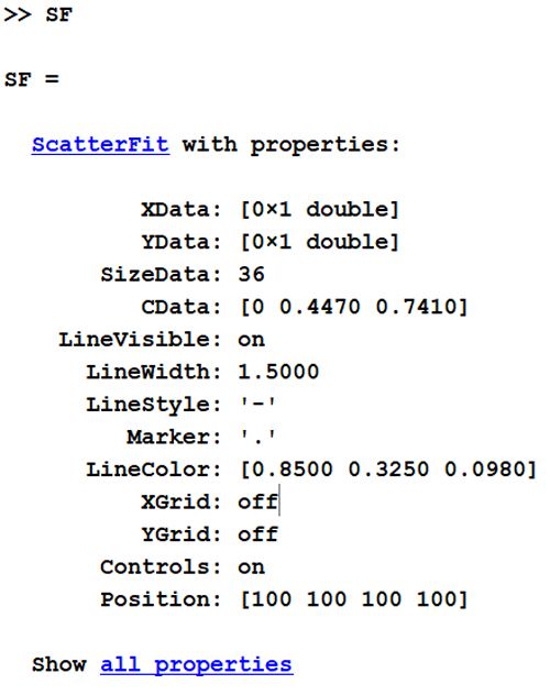
Figure 5. ScatterFit chart API.
Users can access or modify these properties using the sample syntax in Table 1. The associated chart graphics update dynamically in response to property modifications. For example, changing the LineWidth property of the chart updates the LineWidth of the best-fit line.
We implement parts of the chart’s API using Dependent properties. A Dependent property is one whose value is not stored explicitly, but rather is derived from other properties in the class. In a chart, the Dependent properties depend on private properties such as the low-level graphics or internal data properties.
To define a Dependent property, we first declare its name in a properties block with attribute Dependent. This indicates that the property’s value depends on other properties within the class.
properties (Dependent)
    % Chart x-data.
    XData(:, 1) double {mustBeReal}
    % Chart y-data.
    YData(:, 1) double {mustBeReal}
end % properties (Dependent)
We also need to specify how the property depends on the other class properties by writing the corresponding get method. This method returns a single output argument – namely, the value of the Dependent property. In the ScatterFit chart, the XData property of the chart (part of the chart’s public interface) is simply the underlying XData_ property, which is stored internally as a private property of the chart.
function value = get.XData(obj)

    value = obj.XData_;

end % get.XData
Each data property also requires a set method. This assigns the user-specified value to the correct internal chart property and triggers any necessary graphics updates.
For the ScatterFit chart, we support dynamic modifications (including length changes) to the data properties (XData and YData). When the user sets the (public) XData of the chart, we either pad or truncate the opposite (private) data property YData_, depending on whether the new data vector is respectively longer or shorter than the existing data. Recall that this set method will be invoked on construction if the user has specified XData when creating the chart.
function set.XData(obj, value)

    % Mark the chart for an update.
    obj.ComputationRequired = true();

    % Decide how to modify the chart data.
    nX = numel(value);
    nY = numel(obj.YData_);

    if nX < nY % If the new x-data is too short then truncate the chart y-data.
        obj.YData_ = obj.YData_(1:nX);
    else
        % Otherwise, if nX >= nY, then pad the y-data.
        obj.YData_(end+1:nX, 1) = NaN;
    end % if

    % Set the internal x-data.
    obj.XData_ = value;

end % set.XData
Note that the chart’s update method is invoked automatically whenever the user sets a public property. To avoid unnecessary and time-consuming calculations, we use a private, internal logical property ComputationRequired to record, in the set methods, whether a full update is necessary.
Public API properties that do not require new computation when they change do not need a get or set method. Instead, we simply refresh the corresponding internal objects at the end of the update method. Typically, public API properties include decorative and cosmetic aspects of the chart such as colors, line widths, and styles, which are inexpensive to update.
In the ScatterFit chart, the update method contains the code necessary to set the new data in the Scatter object, recompute the best-fit line and set the new data in the corresponding Line object.
function update( obj )

    if obj.ComputationRequired

    % Update the scatter series with the new data.
    set(obj.ScatterSeries, "XData", obj.XData_, "YData", obj.YData_)

    % Obtain the new best-fit line.
    m = fitlm(obj.XData_, obj.YData_);

    % Update the best-fit line graphics.
    [~, posMin] = min(obj.XData_);
    [~, posMax] = max(obj.XData_);
    set(obj.BestFitLine, "XData", obj.XData_([posMin, posMax]), "YData", m.Fitted([posMin, posMax]))

    % Mark the chart clean.
    obj.ComputationRequired = false();

    end % if

    % Refresh the chart's decorative properties.
    set(obj.ScatterSeries, "CData", obj.CData, "SizeData", obj.SizeData)

end % update
We implement the set method for YData in an identical way, switching the roles of the X/YData properties.
To create a rich API appropriate for end users, we implement a broad set of public properties. Note that standard properties such as Parent, Position, Units, and Visible are all inherited from the superclass and do not require additional implementation in the chart.
Adding Chart Annotation Methods
In the API, we provide familiar and easy-to-use methods for annotating the chart. These annotation methods overload (have the same name as) the corresponding high-level graphics decoration function. To use these methods, the user provides a reference to the chart as the first input argument, followed by inputs to the decoration function.
xlabel(SF, "x-data", "FontSize", 12)
If supported by the decoration function, the annotation method can also be called with an output to return a reference to the graphics object for further customization. For example, the xlabel function returns a text object.
xl = xlabel(SF, "x-data");
To support name-value pairs and output arguments, it is convenient to use the cell arrays varargin and varargout. The syntax varargin{:} produces a comma-separated list of the input arguments. We determine the number of outputs from the caller using nargout. To handle a variable number of output arguments (typically, 0 or 1 for these methods) we use the syntax [varargout{1:nargout}] when invoking the decoration function. A typical annotation method has the following structure:
function varargout = xlabel(obj, varargin)

    [varargout{1:nargout}] = xlabel(obj.Axes, varargin{:});

end % xlabel
Including Interactive Controls in Charts
In addition to the chart’s API, we can include controls that provide end users with options for chart interaction and modification (Figure 6).
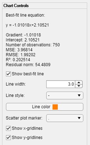
Figure 6. Examples of interactive chart controls.
We initialize these controls in the chart setup method, using components for app building. Each control has a callback function, implemented as a private method. This method has three input arguments:
- The chart object.
- A reference to the source object (the object responsible for triggering the callback)—in this case, the source object is the corresponding user control.
- Event data. This is an object automatically passed to the callback function by MATLAB when the user interacts with the control. The event data object contains additional information about the event.
For example, consider the callback function for the checkbox controlling the visibility of the best-fit line. This function toggles the visibility of the underlying line object based on the value of the checkbox.
function toggleLineVisibility(obj, s, ~)
%TOGGLELINEVISIBILITY Toggle the visibility of the best-fit line.

    obj.BestFitLine.Visible = s.Value;

end % toggleLineVisibility
The values of each control must be synchronized with the corresponding chart property. To achieve this, we equip the chart property with the Dependent attribute and then implement its get and set methods. Note that in addition to updating the internal graphics object, the set method must also update the value of the control object.
The code corresponding to the best-fit line visibility is shown below. To ensure compatibility between the property and checkbox values, we convert the property to the matlab.lang.OnOffSwitchState type. This type supports any compatible syntax for representing true and false values, such as 1 and 0, as well as "on" and "off".
properties (Dependent)
    % Visibility of the best-fit line.
    LineVisible(1, 1) matlab.lang.OnOffSwitchState
end % properties (Dependent)

function value = get.LineVisible(obj)

value = obj.BestFitLine.Visible;

end % get.LineVisible

function set.LineVisible(obj, value)

% Update the property.
obj.BestFitLine.Visible = value;
% Update the check box.
obj.BestFitLineCheckBox.Value = value;

end % set.LineVisible
Integrating Charts with App Designer
As of MATLAB R2021a, charts developed using the ComponentContainer superclass can be integrated with App Designer (Figure 7). With App Designer you can share charts with end users by creating metadata. The installed chart will then appear in the user’s App Designer Component Library, where it can be used interactively in the canvas like any other component.
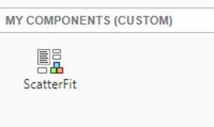
Figure 7. Custom chart integrated with App Designer.
Summary
In this article, we described design patterns and best practices for the implementation of custom charts, using the ScatterFit chart as an example. Many common visualization tasks, especially those that require dynamic graphics, can be performed using an appropriate chart. Designing and creating a chart requires up-front development time and effort, but charts can substantially simplify many visualization workflows.
Published 2021