Train Transformer Autoencoder for Eigenvector-based CSI Feedback Compression

Since R2026a

This example uses:

This example shows how to train an autoencoder neural network with a transformer backbone to compress downlink channel state information (CSI) over a clustered delay line (CDL) channel.

In this example, you:

Define and Train Neural Network Model with a transformer backbone for CSI feedback autoencoding.
Test Network accuracy and the Effect of Quantized Codewords on the system performance.

Type I and Type II codebooks specified in 3GPP Release 15 are based on implicit CSI feedback where the UE performs singular value decomposition (SVD) on downlink CSI matrix to extract the eigen vectors to form the precoding matrix. The precoding matrix is used to search predefined codebooks to select the precoding matrix indicator (PMI) which the UE transmits to the gNB. 3GPP Release 19 investigated the use case of DL-based CSI feedback based on the existing mechanism of using implicit feedback where neural networks replace the PMI modules at the UE and the gNB. Compared to CNN autoencoders, transformer networks can exploit long-term dependencies in data samples by using a self-attention mechanism. For CSI feedback, a transformer network can outperform a CNN in capturing the channel features across frequency subcarriers and transmit antennas.

In this example, you design and train an autoencoder with a transformer backbone for eigenvector based CSI feedback (implicit CSI feedback [3]) compression. The UE forms the precoding matrix and uses the encoder network to generate PMI for feedback. Correspondingly, the gNB uses the decoder network to reconstruct the precoding matrix based on the received PMI.

AI Workflow for CSI Feedback

Steps in this AI-based CSI feedback workflow include data generation, data preparation, and model training. You can run each step independently or work through the steps in order. Train Model is the focus of this example.

For a description of the CSI feedback process and AI workflow, see AI-Based CSI Feedback. Briefly, the workflow steps are:

1. Generate Data - Generate channel estimate data, as shown in the Generate MIMO OFDM Channel Realizations for AI-Based Systems example.

2. Prepare Data - Data preparation, as shown in the Preprocess Data for AI Eigenvector-Based CSI Feedback Compression example.

3. Train Model - Model training inputs preprocessed channel estimate data to neural networks to reconstruct CSI data, which begins in the Define and Train Neural Network Model section of this example.

For a list of additional examples that train, compress, and test autoencoder models, see the Further Exploration section.

Define and Train Neural Network Model

If the required data is not present in the workspace, generate and prepare the data. After preprocessing the data, you can view the system configuration by inspecting outputs (inputData, systemParams, dataOptions, channel, and carrier) of the prepareData function.

if ~exist("inputData","var") || ~exist("systemParams","var") ...
        || ~exist("dataOptions","var") || ~exist("channel","var") ...
        || ~exist("carrier","var")
    numSamples = 10000;
[inputData,systemParams,dataOptions,channel,carrier] = ...
prepareData(numSamples);
end

Starting parallel pool (parpool) using the 'Processes' profile ...
21-Jan-2026 16:33:19: Job Queued. Waiting for parallel pool job with ID 1 to start ...
Connected to parallel pool with 6 workers.
Removing invalid data directory: C:\Users\user\OneDrive - MathWorks\Documents\MATLAB\ExampleManager\user.Bdoc.j3141665\deeplearning_shared-ex97974439\Data
Starting channel realization generation
6 worker(s) running
00:03:45 - 100% Completed
Starting CSI data preprocessing
6 worker(s) running
00:01:55 - 100% Completed

Define Model Variables

Initialize variables that define the neural network model inputs. The inputDataMat variable contains $N_{s a m p l e s}$ samples of $N_{t x I Q}$ -by- $N_{s b}$ arrays.

inputDataMat = inputData{1};
[NtxIQ,Nsb,Nsamples] = size(inputDataMat)

NtxIQ = 
64

Nsb = 
12

Nsamples = 
10000

Partition the data into training, validation and testing sets.

N = size(inputDataMat,3);
numTrain = floor(N*0.8)

numTrain = 
8000

numVal = floor(N*0.1)

numVal = 
1000

numTest = floor(N*0.1)

numTest = 
1000

inputDataT = inputDataMat(:,:,1:numTrain);
inputDataV = inputDataMat(:,:,numTrain+(1:numVal));
inputDataTest = inputDataMat(:,:,numTrain+numVal+(1:numTest));

Design Eigenvector CSI Transformer Network

Use the helperEVCSICreateNetwork function to create an EVCSINet network, which follows [3]:

Specify the network input size as the number of transmit antennas by the number of subbands.
Specify the linear and positional embedding dimension for each subband as the model dimension.
Specify the number of basic blocks for the encoder and decoder. Each basic block consists of a multi-headed self-attention block and a feed-forward block.
Specify the number of heads for the self-attention blocks.
Specify the feed-forward dimension and dropout probability for the feed-forward blocks.
Specify the PMI vector size before quantization.

inputSize = [NtxIQ, Nsb, NaN];
modelDimension = 128;
numBasicBlocks = 2;
feedforwardDimension = modelDimension*4;
dropoutProbability = 0.1;
numAttentionHeads = 8;
encoderOutputSize = 60;

EVCSINet = helperEVCSICreateNetwork(inputSize, ...
    modelDimension, ...
    feedforwardDimension, ...
    dropoutProbability, ...
    numAttentionHeads, ...
    numBasicBlocks, ...
    encoderOutputSize, ...
    Nsb);

analyzeNetwork(EVCSINet)

Explore Network

To explore the network, you can visualize it by using the Deep Network Designer (Deep Learning Toolbox) app.

deepNetworkDesigner(EVCSINet)

The network consists of a set of main components in networkLayer (Deep Learning Toolbox) objects. To view the contents of a network layer, double-click the layer in Deep Network Designer.

An autoencoder network consists of two parts: an encoder and a decoder. The encoder includes an embedding block, numBasicBlocks basic blocks, and the PMI mapping block. The decoder includes numBasicBlocks basic blocks, and the PMI demapping block.

Embedding Layers

The linear embedding layer converts the channel response across the transmit antennas to a dense learnable representation of size modelDimension. The positional encoder injects information about the index of the channel response at each transmit antenna with respect to all antennas in the input array.

Basic Block

The basic block consists of a multi-headed self-attention block followed by a feed-forward network. The self-attention block computes attention scores between the channel response of all pairs of transmit antennas, which helps the model capture the dependency across all transmit antennas. The feed-forward block adds nonlinearity and increases the model representation capability after mixing the attention scores. The residual connection between the input and the output of the feed-forward block helps the gradient flow and makes the model easier to train.

PMI Mapping and Demapping

The mapping block projects the output of the last basic block to a lower dimension PMI vector and the geluLayer (Deep Learning Toolbox) normalizes the encoder output. The Gelu layer marks the last layer of the encoder. The demapping block projects the PMI codeword back to a higher dimension for the decoder to reconstruct the eigen vector for each subband. It starts with a fully connected layer.

Train Deep Neural Network

Set the training options for the autoencoder neural network and train the network using the trainnet (Deep Learning Toolbox) function. Training takes about 2 hours on an AMD® EPYC 7262 CPU @ 3.20GHz with 8 NVIDIA GeForce RTX A5000 GPUs. Set trainNow to false to load the pretrained network. The saved network works for the following settings. If you change any of these settings, set trainNow to true. Adjust the saveNetwork flag to save the trained network. See Antenna Array for details on the antenna array configuration.

The pretrained model used 80,000 training samples and 10,000 validation samples.

txAntennaSize = [4 4 2 1 1]; % rows, columns, polarizations, panels
rxAntennaSize = [2 2 1 1 1]; % rows, columns, polarizations, panels
rmsDelaySpread = 300e-9;     % s
maxDoppler = 1;              % Hz
nSizeGrid = 48;              % Number resource blocks (RB)
                             % 12 subcarriers per RB
subcarrierSpacing = 15;

trainNow = false;
saveNetwork = false;
epochs = 1000;
batchSize = 1000;
initLearnRate = 1e-4;
valFreq = 120; % iterations

A warm-up period in the beginning of training a transformer network helps the network converge to a better local solution. To use a custom sequence of training schedules, create a cell array containing the warmupLearnRate (Deep Learning Toolbox) object followed by the built-in cosine learning rate schedule. For information about learning rate schedules, see the trainingOptions (Deep Learning Toolbox) function. Use the local helper function helperMeanCosineSimilarity as the training loss function.

schedule = {warmupLearnRate( ...
    NumSteps=30, ...
    FrequencyUnit="epoch"), ...
    "cosine"
    };

options = trainingOptions("adam", ...
    InitialLearnRate=initLearnRate, ...
    LearnRateSchedule=schedule, ...
    MaxEpochs=epochs, ...
    MiniBatchSize=batchSize, ...
    Shuffle="every-epoch", ...
    ValidationFrequency=valFreq, ...
    ValidationData={inputDataV,inputDataV}, ...
    Verbose=false, ...
    OutputNetwork="auto", ...
    Plots="training-progress", ...
    ExecutionEnvironment="auto", ...
    InputDataFormats="CTB", ...
    TargetDataFormats="CTB", ...
    ValidationPatience=20);

if trainNow
    [trainedNet, trainInfo] = trainnet(inputDataT,inputDataT,EVCSINet,@(x,t) -helperMeanCosineSimilarity(x,t),options); %#ok
    if saveNetwork
        save("trainedNetwork_" ...
            + string(datetime("now","Format","dd_MM_HH_mm")), 'trainedNet')
    end
else
    load("trainedNet.mat","trainedNet")
end

Test Network

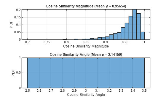
Test the accuracy of the trained network over the test data set by using the testnet (Deep Learning Toolbox) function. Create a cell array of metric functions to compute the average value of each metric over the test samples. The NMSE in dB and the cosine similarity coefficient are typical metrics to evaluate the CSI feedback and recovery performance. Use the local function helperMeanCosineSimilarity as metrics for the testnet function.

testResults = testnet(trainedNet,inputDataTest,inputDataTest,@(x,t) helperMeanCosineSimilarity(x,t), ...
InputDataFormats="CTB",TargetDataFormats="CTB")

testResults = 
0.9564

cossim = zeros(numTest,1);
xHat = predict(trainedNet,inputDataTest);
for n=1:numTest
    % Transpose to compute the 
    in = inputDataTest(:,:,n)';
    out = xHat(:,:,n)';

    % Calculate correlation
    cossim(n) = helperComplexCosineSimilarity(in,out);
end
figure
tiledlayout
nexttile
histogram(abs(cossim),"Normalization","probability")
grid on
title(sprintf("Cosine Similarity Magnitude (Mean \\rho = %1.5f)", ...
mean(abs(cossim))))
xlabel("Cosine Similarity Magnitude"); ylabel("PDF")
nexttile
histogram(angle(cossim),"Normalization","probability")
grid on
title(sprintf("Cosine Similarity Angle (Mean \\rho = %1.5f)", ...
mean(angle(cossim))))
xlabel("Cosine Similarity Angle"); ylabel("PDF")

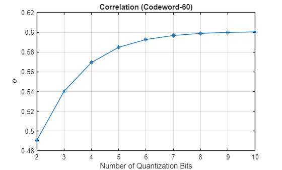
Figure contains 2 axes objects. Axes object 1 with title Cosine Similarity Magnitude (Mean rho = 0 . 95654 ), xlabel Cosine Similarity Magnitude, ylabel PDF contains an object of type histogram. Axes object 2 with title Cosine Similarity Angle (Mean rho = 3 . 14159 ), xlabel Cosine Similarity Angle, ylabel PDF contains an object of type histogram.

Effect of Quantized Codewords

Practical systems require quantizing the encoded codeword by using a small number of bits. Simulate the effect of quantization across the range of [2, 10] bits. Split the trained network into an encoder and a decoder and insert the quantizer/dequantizer between them. The Gelu layer marks the last layer of the encoder.

[encNet,decNet] = helperEVCSIsplitEncoderDecoder(trainedNet,"pmi_mapping:gelu");
codeword = minibatchpredict(encNet,inputDataTest);

Hev = permute(inputDataTest,[2,1,3]);

idxBits = 1;
nBitsVec = 2:10;
rhoQ = zeros(1,length(nBitsVec));

for numBits = nBitsVec
disp("Running for " + numBits + " bit quantization")

    % Quantize between 0:2^n-1 to get bits
    qCodeword = uencode(double(codeword*2-1),numBits);

    % Get back the floating point, quantized numbers
    codewordRx = (single(udecode(qCodeword,numBits))+1)/2;
    HevHat = minibatchpredict(decNet,codewordRx);
    rhoQ(numBits-1) = mean(abs(helperComplexCosineSimilarity(Hev,HevHat)));
    idxBits = idxBits + 1;
end

Running for 2 bit quantization
Running for 3 bit quantization
Running for 4 bit quantization
Running for 5 bit quantization
Running for 6 bit quantization
Running for 7 bit quantization
Running for 8 bit quantization
Running for 9 bit quantization
Running for 10 bit quantization

figure
plot(nBitsVec,rhoQ,'*-')
title("Correlation (Codeword-" + size(codeword,2) + ")")
xlabel("Number of Quantization Bits"); ylabel("\rho")
grid on

Figure contains an axes object. The axes object with title Correlation (Codeword-60), xlabel Number of Quantization Bits, ylabel rho contains an object of type line.

Further Exploration

To explore other task-specific processes, see these examples:

CSI Feedback with Transformer Autoencoder — Design, train, and evaluate a transformer autoencoder for full CSI compression and reconstruction.
Optimize CSI Feedback Autoencoder Training Using MATLAB Parallel Server and Experiment Manager — Accelerate determining the optimal training hyperparameters of an autoencoder model that simulates CSI compression by using a MATLAB® Parallel Server™ and the Experiment Manager app.
CSI Feedback with Autoencoders Implemented on an FPGA (Deep Learning HDL Toolbox) — Deploy an implemented CSI autoencoder to an FPGA by using the Deep Learning HDL Toolbox™.

You can also explore how to train and test PyTorch™ and Keras™ based neural networks hosted by MATLAB®:

Helper Functions

helper3GPPChannelRealizations

helperPreprocess3GPPChannelData

helperEVCSIPartitionData

helperEVCSIBasicBlock

helperEVCSICreateNetwork

helperEVCSIQuantizationLayer

helperComplexCosineSimilarity

Local Functions

function [inputData,systemParams,dataOptions,channel,carrier] = prepareData(numSamples)

systemParams.TxAntennaSize = [4 4 2 1 1];   % rows, columns, polarization, panels
systemParams.RxAntennaSize = [2 2 1 1 1];   % rows, columns, polarization, panels
systemParams.MaxDoppler = 1;                % Hz
systemParams.RMSDelaySpread = 300e-9;       % s
systemParams.DelayProfile = "CDL-C"; % CDL-A, CDL-B, CDL-C, CDL-D, CDL-D, CDL-E

carrier = nrCarrierConfig;
nSizeGrid = 48;                                         % Number resource blocks (RB)
systemParams.SubcarrierSpacing = 15;  % 15, 30, 60, 120 kHz
carrier.NSizeGrid = nSizeGrid;
carrier.SubcarrierSpacing = systemParams.SubcarrierSpacing;
waveInfo = nrOFDMInfo(carrier);

channel = nrCDLChannel;
channel.DelayProfile = systemParams.DelayProfile;
channel.DelaySpread = systemParams.RMSDelaySpread;     % s
channel.MaximumDopplerShift = systemParams.MaxDoppler; % Hz
channel.RandomStream = "Global stream";
channel.TransmitAntennaArray.Size = systemParams.TxAntennaSize;
channel.ReceiveAntennaArray.Size = systemParams.RxAntennaSize;
channel.ChannelFiltering = false;
channel.SampleRate = waveInfo.SampleRate;
channel.CarrierFrequency = 3.5e9;

samplesPerSlot = ...
    sum(waveInfo.SymbolLengths(1:waveInfo.SymbolsPerSlot));
slotsPerFrame = 1;
channel.NumTimeSamples = samplesPerSlot*slotsPerFrame;
systemParams.NumSymbols = slotsPerFrame*14;
useParallel = true;
saveData =  true;
dataDir = fullfile(pwd,"Data");
dataFilePrefix = "nr_channel_est";
resetChanel = true;
sdsChan = helper3GPPChannelRealizations(...
    numSamples, ...
    channel, ...
    carrier, ...
    UseParallel=useParallel, ...
    SaveData=saveData, ...
    DataDir=dataDir, ...
    dataFilePrefix=dataFilePrefix, ...
    NumSlotsPerFrame=slotsPerFrame, ...
    ResetChannelPerFrame=resetChanel);

[inputData,dataOptions] = helperPreprocess3GPPChannelData( ...
    sdsChan, ...
    TrainingObjective="eigenvector autoencoding", ...
    DataComplexity="complex", ...
    Verbose=true, ...
    SaveData=false, ...
    UseParallel=true);
end

function meanRho = helperMeanCosineSimilarity(x,xHat)
%HELPERMEANCOSINESIMILARITY Cosine similarity coefficient

% Permute x & xHat to compute the cosine similarity between eigenvector of
% each subband
xpermute = permute(stripdims(x), [2,1,3]);
xHatpermute = permute(stripdims(xHat), [2,1,3]);

% Compute the average cosine similarity over subcarriers
rhoPerSample = helperComplexCosineSimilarity(xpermute,xHatpermute);
meanRho = mean(abs(rhoPerSample));
end

References

[1] 3GPP TS 38.214. “NR; Physical layer procedures for data.” 3rd Generation Partnership Project; Technical Specification Group Radio Access Network.

[2] 3GPP TR 38.843. “Study on Artificial Intelligence (AI)/Machine Learning (ML) for NR Air Interface.” 3rd Generation Partnership Project; Technical Report Group Radio Access Network.

[3] Han, X., Zhiqin, W., Dexin, L., Wenqiang, T., Xiaofeng, L., Wendong, L., Shi, J., Jia, S., Zhi, Z. and Ning, Y., 2024. AI enlightens wireless communication: A transformer backbone for CSI feedback. China Communications.