Training and Testing a Neural Network for LLR Estimation

This example uses:

This example shows how to generate signals and channel impairments to train a neural network, called LLRNet, to estimate exact log likelihood ratios (LLR).

Most modern communication systems, such as 5G New Radio (NR) and Digital Video Broadcasting for Satellite, Second Generation (DVB-S.2) use forward error correction algorithms that benefit from soft demodulated bit values. These systems calculate soft bit values using the LLR approach. LLR is defined as the log of the ratio of probability of a bit to be 0 to the probability of a bit to be 1 or

$l_{i} ≜ \log (\frac{P_{r} (c_{i} = 0 | s_{}^{ˆ})}{P_{r} (c_{i} = 1 | s_{}^{ˆ})})$ , $i = 1, . . ., k$

where $s_{}^{ˆ}$ is an k-bit received symbol, and $c_{i}$ is the $i^{t h}$ bit of the symbol. Assuming an additive white Gaussian noise (AWGN) channel, the exact computation of the LLR expression is

$l_{i} ≜ \log (\frac{\sum_{s \in c_{i}^{0}} \exp (- \frac{‖ s_{}^{ˆ} - s ‖_{2}^{2}}{σ^{2}})}{\sum_{s \in c_{i}^{1}} \exp (- \frac{‖ s_{}^{ˆ} - s ‖_{2}^{2}}{σ^{2}})})$

where $σ^{2}$ is the noise variance. Exponential and logarithmic calculations are very costly especially in embedded systems. Therefore, most practical systems use the max-log approximation. For a given array $x$ , the max-log approximation is

$\log (\sum_{j} \exp (- x_{j}^{2})) \approx \max_{j} (- x_{j}^{2})$ .

Substituting this in the exact LLR expression results in the max-log LLR approximation [1]

$l_{i} \approx \frac{1}{σ^{2}} (\min_{s \in C_{i}^{1}} ‖ s_{}^{ˆ} - s ‖_{2}^{2} - \min_{s \in C_{i}^{0}} ‖ s_{}^{ˆ} - s ‖_{2}^{2})$ .

LLRNet uses a neural network to estimate the exact LLR values given the baseband complex received symbol for a given SNR value. A shallow network with a small number of hidden layers has the potential to estimate the exact LLR values at a complexity similar to the approximate LLR algorithm [1].

Compare Exact LLR, Max-Log Approximate LLR and LLRNet for M-ary QAM

5G NR uses M-ary QAM modulation. This section explores the accuracy of LLRNet in estimating the LLR values for 16-, 64-, and 256-QAM modulation. Assume an M-ary QAM system that operates under AWGN channel conditions. This assumption is valid even when the channel is frequency selective but symbols are equalized. The following shows calculated LLR values for the following three algorithms:

Exact LLR
Max-log approximate LLR
LLRNet

16-QAM LLR Estimation Performance

Calculate exact and approximate LLR values for symbol values that cover the 99.7% ( $\pm 3 σ$ ) of the possible received symbols. Assuming AWGN, 99.7% ( $\pm 3 σ$ ) of the received signals will be in the range $[\max_{s \in C} (R e (s) + 3 σ) \min_{s \in C} (R e (s) - 3 σ)] + i [\max_{s \in C} (I m (s) + 3 σ) \min_{s \in C} (I m (s) - 3 σ)]$ . Generate uniformly distributed I/Q symbols over this space and use qamdemod function to calculate exact LLR and approximate LLR values.

M = 16;             % Modulation order
k = log2(M);        % Bits per symbols
SNRValues = -5:5:5; % in dB
numSymbols = 1e4;
numSNRValues = length(SNRValues);
symOrder = llrnetQAMSymbolMapping(M);

const = qammod(0:15,M,symOrder,'UnitAveragePower',1);
maxConstReal = max(real(const));
maxConstImag = max(imag(const));

numBits = numSymbols*k;
exactLLR = zeros(numBits,numSNRValues);
approxLLR = zeros(numBits,numSNRValues);
rxSym = zeros(numSymbols,numSNRValues);
for snrIdx = 1:numSNRValues
    SNR = SNRValues(snrIdx);
    noiseVariance = 10^(-SNR/10);
    sigma = sqrt(noiseVariance);
    
    maxReal = maxConstReal + 3*sigma;
    minReal = -maxReal;
    maxImag = maxConstImag + 3*sigma;
    minImag = -maxImag;
    
    r = (rand(numSymbols,1)*(maxReal-minReal)+minReal) + ...
        1i*(rand(numSymbols,1)*(maxImag-minImag)+minImag);
    rxSym(:,snrIdx) = r;
    
    exactLLR(:,snrIdx) = qamdemod(r,M,symOrder,...
        'UnitAveragePower',1,'OutputType','llr','NoiseVariance',noiseVariance);
    approxLLR(:,snrIdx) = qamdemod(r,M,symOrder,...
        'UnitAveragePower',1,'OutputType','approxllr','NoiseVariance',noiseVariance);
end

Set Up and Train Neural Network

Set up a shallow neural network with one input layer, one hidden layer, and one output layer. Input a received symbol to the network and train it to estimate the exact LLR values. Since the network expects real inputs, create a two column vector, where the first column is the real values of the received symbol and the second column is the imaginary values of the received symbol. Also, the output must be a $k \times N$ vector, where $k$ is the number of bits per symbol and $N$ is the number of symbols.

nnInput = zeros(numSymbols,2,numSNRValues);
nnOutput = zeros(numSymbols,k,numSNRValues);
for snrIdx = 1:numSNRValues
    rxTemp = rxSym(:,snrIdx);
    rxTemp = [real(rxTemp) imag(rxTemp)];
    nnInput(:,:,snrIdx) = rxTemp;
    
    llrTemp = exactLLR(:,snrIdx);
    nnOutput(:,:,snrIdx) = reshape(llrTemp, k, numSymbols)';
end

For 16-QAM symbols, the hidden layer has 8 neurons and the output layer has 4 neurons, which corresponds to the number of bits per symbol. The llrnetNeuralNetwork helper function returns a preconfigured neural network. Train the neural network for three different SNR values. Use the exact LLR values calculated using the qamdemod function as the expected output values.

hiddenLayerSize = 8;
trainedNetworks = cell(1,numSNRValues);
for snrIdx=1:numSNRValues
    fprintf('Training neural network for SNR = %1.1fdB\n', ...
        SNRValues(snrIdx))
    x = nnInput(:,:,snrIdx)';
    y = nnOutput(:,:,snrIdx)';
    
    MSExactLLR = mean(y(:).^2);
    fprintf('\tMean Square LLR = %1.2f\n', MSExactLLR)
    
    % Train the Network. Use parallel pool, if available. Train three times
    % and pick the best one.
    mse = inf;
    for p=1:3
        netTemp = llrnetNeuralNetwork(hiddenLayerSize);
        if parallelComputingLicenseExists()
            [netTemp,tr] = train(netTemp,x,y,'useParallel','yes');
        else
            [netTemp,tr] = train(netTemp,x,y);
        end
        % Test the Network
        predictedLLRSNR = netTemp(x);
        mseTemp = perform(netTemp,y,predictedLLRSNR);
        fprintf('\t\tTrial %d: MSE = %1.2e\n', p, mseTemp)
        if mse > mseTemp
            mse = mseTemp;
            net = netTemp;
        end
    end
    
    % Store the trained network
    trainedNetworks{snrIdx} = net;
    fprintf('\tBest MSE = %1.2e\n', mse)
end

Training neural network for SNR = -5.0dB

	Mean Square LLR = 4.43

Starting parallel pool (parpool) using the 'Processes' profile ...
19-Jul-2024 15:25:01: Job Queued. Waiting for parallel pool job with ID 1 to start ...
Connected to parallel pool with 6 workers.

		Trial 1: MSE = 7.44e-05
		Trial 2: MSE = 6.90e-05
		Trial 3: MSE = 6.81e-05

	Best MSE = 6.81e-05

Training neural network for SNR = 0.0dB

	Mean Square LLR = 15.74

		Trial 1: MSE = 1.86e-03
		Trial 2: MSE = 4.04e-04
		Trial 3: MSE = 9.05e-05

	Best MSE = 9.05e-05

Training neural network for SNR = 5.0dB

	Mean Square LLR = 60.01

		Trial 1: MSE = 8.59e-03
		Trial 2: MSE = 2.19e-02
		Trial 3: MSE = 2.14e-02

	Best MSE = 8.59e-03

Performance metric for this network is mean square error (MSE). The final MSE values show that the neural network converges to an MSE value that is at least 40 dB less than the mean square exact LLR values. Note that, as SNR increases so do the LLR values, which results in relatively higher MSE values.

Results for 16-QAM

Compare the LLR estimates of LLRNet to that of exact LLR and approximate LLR. Simulate 1e4 16-QAM symbols and calculate LLR values using all three methods. Do not use the symbols that we generated in the previous section so as not to give LLRNet an unfair advantage, since those symbols were used to train the LLRNet.

numBits = numSymbols*k;
d = randi([0 1], numBits, 1);

txSym = qammod(d,M,symOrder,'InputType','bit','UnitAveragePower',1);

exactLLR = zeros(numBits,numSNRValues);
approxLLR = zeros(numBits,numSNRValues);
predictedLLR = zeros(numBits,numSNRValues);
rxSym = zeros(length(txSym),numSNRValues);
for snrIdx = 1:numSNRValues
    SNR = SNRValues(snrIdx);
    sigmas = 10^(-SNR/10);
    r = awgn(txSym,SNR);
    rxSym(:,snrIdx) = r;
    
    exactLLR(:,snrIdx) = qamdemod(r,M,symOrder,...
        'UnitAveragePower',1,'OutputType','llr','NoiseVariance',sigmas);
    approxLLR(:,snrIdx) = qamdemod(r,M,symOrder,...
        'UnitAveragePower',1,'OutputType','approxllr','NoiseVariance',sigmas);
    
    net = trainedNetworks{snrIdx};
    x = [real(r) imag(r)]';
    tempLLR = net(x);
    predictedLLR(:,snrIdx) = reshape(tempLLR, numBits, 1);
end

qam16Results.exactLLR = exactLLR;
qam16Results.approxLLR = approxLLR;
qam16Results.predictedLLR = predictedLLR;
qam16Results.RxSymbols = rxSym;
qam16Results.M = M;
qam16Results.SNRValues = SNRValues;
qam16Results.HiddenLayerSize = hiddenLayerSize;
qam16Results.NumSymbols = numSymbols;

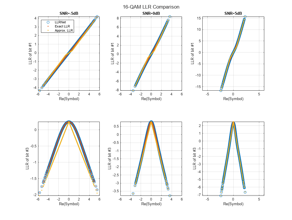
The following figure shows exact LLR, max-log approximate LLR, and LLRNet estimate of LLR values versus the real part of the received symbol for odd bits. LLRNet matches the exact LLR values even for low SNR values.

llrnetPlotLLR(qam16Results,'16-QAM LLR Comparison')

64-QAM and 256-QAM LLR Estimation Performance

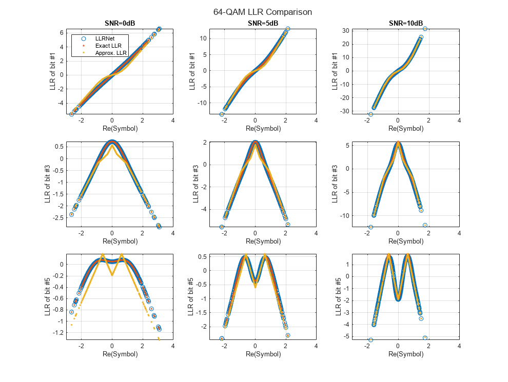
Check if the LLRNet can estimate the LLR values for higher order QAM. Repeat the same process you followed for 16-QAM for 64-QAM and 256-QAM using the llrnetQAMLLR helper function. The following figures show exact LLR, max-log approximate LLR, and LLRNet estimate of LLR values versus the real part of the received symbol for odd bits.

trainNow = false;
if trainNow
    % Parameters for 64-QAM
    simParams(1).M = 64; %#ok<UNRCH>
    simParams(1).SNRValues = 0:5:10;
    simParams(1).HiddenLayerSize = 16;
    simParams(1).NumSymbols = 1e4;
    simParams(1).UseReLU = false;
    
    % Parameters for 256-QAM
    simParams(2).M = 256;
    simParams(2).SNRValues = 0:10:20;
    simParams(2).HiddenLayerSize = 32;
    simParams(2).NumSymbols = 1e4;
    simParams(2).UseReLU = false;
    
    simResults = llrnetQAMLLR(simParams);
    llrnetPlotLLR(simResults(1),sprintf('%d-QAM LLR Comparison',simResults(1).M))
    llrnetPlotLLR(simResults(2),sprintf('%d-QAM LLR Comparison',simResults(2).M))
else
    load('llrnetQAMPerformanceComparison.mat', 'simResults')
    for p=1:length(simResults)
        llrnetPlotLLR(simResults(p),sprintf('%d-QAM LLR Comparison',simResults(p).M))
    end
end

DVB-S.2 Packet Error Rate

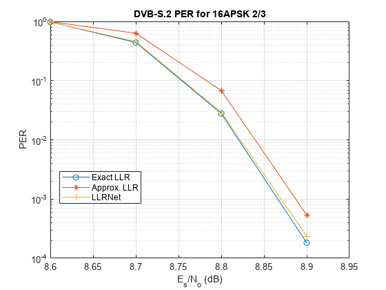
DVB-S.2 system uses a soft demodulator to generate inputs for the LDPC decoder. Simulate the packet error rate (PER) of a DVB-S.2 system with 16-APSK modulation and 2/3 LDPC code using exact LLR, approximate LLR, and LLRNet using llrNetDVBS2PER heper function. The helper function uses the pskdemod function and the dvbsapskdemod (Satellite Communications Toolbox) function to calculate exact and approximate LLR values and the awgn function to simulate the channel.

Set simulateNow to true (or select "Simulate" in the dropdown) to run the PER simulations for the values of subsystemType, EsNoValues, and numSymbols using the llrnetDVBS2PER function. If Parallel Computing Toolbox™ is installed, this function uses the parfor command to run the simulations in parallel. On an Intel® Xeon® W-2133 CPU @ 3.6GHz and running a Run Code on Parallel Pools (Parallel Computing Toolbox) of size 6, the simulation takes about 40 minutes. Set simulateNow to false (or select "Plot saved results" in the dropdown), to load the PER results for the values of subsystemType='16APSK 2/3', EsNoValues=8.6:0.1:8.9, and numSymbols=10000.

Set trainNow to true (or select "Train LLRNet" in the dropdown) to train LLR neural networks for each value of EsNoValues, for the given subsystemType and numSymbols. If Parallel Computing Toolbox is installed, the train function can be called with the optional name-value pair 'useParallel' set to 'yes' to run the simulations in parallel. On an Intel Xeon W-2133 CPU @ 3.6GHz and running a Run Code on Parallel Pools (Parallel Computing Toolbox) of size 6, the simulation takes about 21 minutes. Set trainNow to false (or select "Use saved networks" in the dropdown) to load LLR neural networks trained for subsystemType='16APSK 2/3', EsNoValues=8.6:0.1:8.9.

For more information on the DVB-S.2 PER simulation, see the DVB-S.2 Link, Including LDPC Coding in Simulink example. For more information on training the network, refer to the llrnetTrainDVBS2LLRNetwork function and [1].

simulateNow = false;
if simulateNow
    subsystemType = '16APSK 2/3'; %#ok<UNRCH>
    EsNoValues = 8.6:0.1:8.9;     % in dB
    numFrames = 10000;
    numErrors = 200;
    
    trainNow = false;
    if trainNow && (~strcmp(subsystemType,'16APSK 2/3') || ~isequal(EsNoValues,8.6:0.1:9))
        % Train the networks for each EsNo value
        numTrainSymbols = 1e4;
        hiddenLayerSize = 64;
        llrNets = llrnetTrainDVBS2LLRNetwork(subsystemType, EsNoValues, numTrainSymbols, hiddenLayerSize);
    else
        load('llrnetDVBS2Networks','llrNets','subsystemType','EsNoValues');
    end
    
    % Simulate PER with exact LLR, approximate LLR, and LLRNet
    [perLLR,perApproxLLR,perLLRNet] = llrnetDVBS2PER(subsystemType,EsNoValues,llrNets,numFrames,numErrors);
    llrnetPlotLLRvsEsNo(perLLR,perApproxLLR,perLLRNet,EsNoValues,subsystemType)
else
    load('llrnetDVBS2PERResults.mat','perApproxLLR','perLLR','perLLRNet',...
        'subsystemType','EsNoValues');
    llrnetPlotLLRvsEsNo(perLLR,perApproxLLR,perLLRNet,EsNoValues,subsystemType)
end

Figure contains an axes object. The axes object with title DVB-S.2 PER for 16APSK 2/3, xlabel E indexOf s baseline /N indexOf o baseline blank (dB), ylabel PER contains 3 objects of type line. These objects represent Exact LLR, Approx. LLR, LLRNet.

The results show that the LLRNet almost matches the performance of exact LLR without using any expensive operations such as logarithm and exponential.

Further Exploration

Try different modulation and coding schemes for the DVB-S.2 system. The full list of modulation types and coding rates are given in the DVB-S.2 Link, Including LDPC Coding in Simulink example. You can also try different sizes for the hidden layer of the network to reduce the number of operations and measure the performance loss as compared to exact LLR.

The example uses these helper functions. Examine these files to learn about details of the implementation.

llrnetDVBS2PER.m: Simulate DVB-S.2 PER using exact LLR, approximate LLR, and LLRNet LLR
llrnetTrainDVBS2LLRNetwork.m: Train neural networks for DVB-S.2 LLR estimation
llrnetQAMLLR.m: Train neural networks for M-ary QAM LLR estimation and calculate exact LLR, approximate LLR, and LLRNet LLR
llrnetNeuralNetwork.m: Configure a shallow neural network for LLR estimation

References

[1] O. Shental and J. Hoydis, ""Machine LLRning": Learning to Softly Demodulate," 2019 IEEE Globecom Workshops (GC Wkshps), Waikoloa, HI, USA, 2019, pp. 1-7.