LTV Model of Two-Link Robot

This example uses:

This example shows how to obtain an LTV model of a two-link robot along a prescribed trajectory. The robot model and its corresponding dynamics are based on [1] and [2].

Nonlinear Model

This figure gives the schematics of the two-link planar robot.

The robot configuration is described by the joint angles $θ_{1}$ , $θ_{2}$ and torques $τ_{1}$ , $τ_{2}$ applied at the joints to control the position of the tip. The state vector is

$x (t) = [\begin{array}{c} θ_{1} \\ θ_{2} \\ {\dot{θ}}_{1} (t) \\ {\dot{θ}}_{2} (t) \end{array}]$ .

The following equations describe the robot dynamics.

$[\begin{array}{c} α + 2 β \cos (θ_{2}) & δ + β \cos (θ_{2}) \\ δ + β \cos (θ_{2}) & δ \end{array}] [\begin{array}{c} \ddot{θ_{1}} \\ \ddot{θ_{2}} \end{array}] + [\begin{array}{c} - β \sin (θ_{2}) \dot{θ_{2}} & β \sin (θ_{2}) (\dot{θ_{1}} + \dot{θ_{2}}) \\ β \sin (θ_{2}) \dot{θ_{1}} & 0 \end{array}] [\begin{array}{c} \dot{θ_{1}} \\ \dot{θ_{2}} \end{array}] = [\begin{array}{c} τ_{1} \\ τ_{2} \end{array}]$

Here:

$α = I_{z1} + I_{z2} + m_{1} r_{1}^{2} + m_{2} (l_{1}^{2} + r_{2}^{2})$

$β = m_{2} l_{1} r_{2}$

$δ = I_{z2} + m_{2} r_{2}^{2}$

This example uses the twoLinkInverseKinematics.m script to solve this inverse kinematics problem.

Define the physical parameters.

m1 = 3;         % Mass of link 1, kg
m2 = 2;         % Mass of link 2, kg
L1 = 0.3;       % Length of link 1, meters
L2 = 0.3;       % Length of link 2, meters

Desired Trajectory and Inverse Kinematics

The tip of the arm must follow a prescribed planar trajectory $X (t)$ , $Y (t)$ .

T0 = 0;
Tf = 5;
tref = linspace(T0,Tf,400)';
load XYTrajectory x2ref y2ref
plot( x2ref, y2ref, 'b', 'LineWidth',3,'MarkerSize',10)
xlabel('x (m)');
ylabel('y (m)');
grid on
title('Target Trajectory')

Figure contains an axes object. The axes object with title Target Trajectory, xlabel x (m), ylabel y (m) contains an object of type line.

Solve the inverse kinematics problem for joint angles, joint velocities, and torque inputs corresponding to the motion of the end point of link 2. Use joint angles to compute the trajectory of the tip of link 1.

[x,tau] = twoLinkInverseKinematics(tref,x2ref,y2ref,m1,m2,L1,L2);
x1ref = L1*cos(x(:,1));
y1ref = L1*sin(x(:,1));

Plot the joint angles and torques.

plot(tref,x(:,1),'b',tref,x(:,2),'r','LineWidth',2);
legend('\theta_1','\theta_2','location','Best')
ylabel('Angle (rad)')
xlabel('Time (s)')
grid on;

$Figure contains an axes object. The axes object with xlabel Time (s), ylabel Angle (rad) contains 2 objects of type line. These objects represent \theta_1, \theta_2.$

plot(tref,tau(:,1),'b',tref,tau(:,2),'r','LineWidth',2);
legend('\tau_1','\tau_2','location','Best')
ylabel('Torque (Nm)')
xlabel('Time (s)')
grid on;

$Figure contains an axes object. The axes object with xlabel Time (s), ylabel Torque (Nm) contains 2 objects of type line. These objects represent \tau_1, \tau_2.$

Use a Simscape™ Multibody™ model of the two-link robot to simulate the robot response to the computed torques.

tau1 = tau(:,1);
tau2 = tau(:,2);
xinit = x(1,:)';  % initial state

open_system('TwoLinkRobotSM')

Simulate the model, unpack the results, and verify that the tip follows the desired trajectory.

out = sim('TwoLinkRobotSM','ReturnWorkspaceOutputs', 'on');
tsim = out.xsim.time;
xsim = out.xsim.signals.values;

plotTrajectory(xsim,tref,x1ref,y1ref,x2ref,y2ref,L1,L2)

Figure contains an axes object. The axes object with xlabel x (m), ylabel y (m) contains 8 objects of type line, text. One or more of the lines displays its values using only markers These objects represent desired, simulated.

LTV Model

To build an LTV model of two-link robot along the desired trajectory, take linearization snapshots at 50 evenly distributed times between the start and end of the simulation. Use linearize to obtain linearized models at the corresponding operating conditions.

Specify linearization I/Os.

io = [...
   linio('TwoLinkRobotSM/tau1',1,'input');...
   linio('TwoLinkRobotSM/tau2',1,'input');...
   linio('TwoLinkRobotSM/Mux',1,'output')];

Take snapshot operating points.

tlin = linspace(T0,Tf,50);
op = findop('TwoLinkRobotSM',tlin);

Compute linearizations with offsets.

linOpt = linearizeOptions('StoreOffsets',true);
[G,~,info] = linearize('TwoLinkRobotSM',io,op,linOpt);
G.u = 'tau';
G.y = 'x';
G.SamplingGrid = struct('Time',tlin);

Use ssInterpolant to construct an LTV object from the array of linearized models and associated offsets. The resulting LTV model interpolates the linearized dynamics between the snapshot times tlin.

Gltv = ssInterpolant(G,info.Offsets);
Gltv.StateName

ans = 4x1 cell
    {'TwoLinkRobotSM.Subsystem.Revolute_Joint1.Rz.q'}
    {'TwoLinkRobotSM.Subsystem.Revolute_Joint1.Rz.w'}
    {'TwoLinkRobotSM.Subsystem.Revolute_Joint2.Rz.q'}
    {'TwoLinkRobotSM.Subsystem.Revolute_Joint2.Rz.w'}

The states are ordered differently in the linearization. Use xperm to align the state order with the convention $θ_{1}$ , $θ_{2}$ , ${\dot{θ}}_{1}$ , ${\dot{θ}}_{2}$ .

Gltv = xperm(Gltv,[1 3 2 4]);
Gltv.StateName

ans = 4x1 cell
    {'TwoLinkRobotSM.Subsystem.Revolute_Joint1.Rz.q'}
    {'TwoLinkRobotSM.Subsystem.Revolute_Joint2.Rz.q'}
    {'TwoLinkRobotSM.Subsystem.Revolute_Joint1.Rz.w'}
    {'TwoLinkRobotSM.Subsystem.Revolute_Joint2.Rz.w'}

LTV Model Validation

Simulate the response of this LTV model for the same torque inputs and compare with the results from Simscape Multibody.

Simulate the LTV response to torque profiles.

xltv = lsim(Gltv,[tau1 tau2],tref,xinit);

Compare with Simscape results.

clf 
plot(tsim,xsim(:,1),'b',tref,xltv(:,1),'k--',...
   tsim,xsim(:,2),'r',tref,xltv(:,2),'k:','LineWidth',2);
xlim([0 5])
legend('\theta_1 (Simscape)','\theta_1 (LTV)',...
   '\theta_2 (Simscape)','\theta_2 (LTV)','location','Best')
title('Simulation with Continuous LTV Model')

$Figure contains an axes object. The axes object with title Simulation with Continuous LTV Model contains 4 objects of type line. These objects represent \theta_1 (Simscape), \theta_1 (LTV), \theta_2 (Simscape), \theta_2 (LTV).$

Discretization

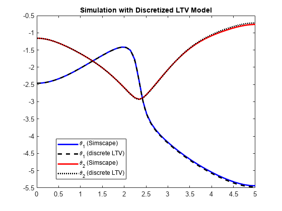
In embedded applications, you often want a discrete model that can be easily simulated. Using c2d, you can compute a Tustin discretization of Gltv and turn it into a discrete gridded LTV model.

Ts = 0.05;
Gd = c2d(Gltv,Ts,'tustin');

Turn Gd into a gridded LTV model with 50 grid points.

k = round(linspace(0,Tf/Ts,50));
Gd = ssInterpolant(Gd,struct('Time',k));

The initial condition for the Tustin discretization is

$z_{0} = x (0) - \frac{T_{s}}{2} \dot{x} (0)$ .

[A,B,~,~,~,dx0,x0,u0] = Gltv.DataFunction(0);
dxinit = dx0+A*(xinit-x0)+B*(tau(1,:)'-u0);
zinit = xinit-Ts/2*dxinit;

Simulate and compare with Simscape results.

t = T0:Ts:Tf;
taud = interp1(tref,[tau1 tau2],t);
xd = lsim(Gd,taud,t,zinit);

clf 
plot(tsim,xsim(:,1),'b',t,xd(:,1),'k--',...
   tsim,xsim(:,2),'r',t,xd(:,2),'k:','LineWidth',2);
xlim([0 5])
legend('\theta_1 (Simscape)','\theta_1 (discrete LTV)',...
   '\theta_2 (Simscape)','\theta_2 (discrete LTV)','location','Best')
title('Simulation with Discretized LTV Model')

$Figure contains an axes object. The axes object with title Simulation with Discretized LTV Model contains 4 objects of type line. These objects represent \theta_1 (Simscape), \theta_1 (discrete LTV), \theta_2 (Simscape), \theta_2 (discrete LTV).$

References

[1] Murray, Richard M., Zexiang Li, and Shankar Sastry. A Mathematical Introduction to Robotic Manipulation. Boca Raton: CRC Press, 1994.

[2] Seiler, Peter, Robert M. Moore, Chris Meissen, Murat Arcak, and Andrew Packard. “Finite Horizon Robustness Analysis of LTV Systems Using Integral Quadratic Constraints.” Automatica 100 (February 2019): 135–43. https://doi.org/10.1016/j.automatica.2018.11.009.