Classify Parkinson's Disease Severity from TDMS Data Using Deep Learning
R2026bThis example shows how to read brain signal recordings from TDMS files, classify Parkinson's disease (PD) severity using a deep learning model, and simulate adaptive deep brain stimulation (DBS).
Adaptive DBS adjusts electrical stimulation delivered to the brain based on symptom severity. The adaptive approach reduces energy use and side effects compared to always-on stimulation. The brain signals are local field potentials (LFPs) recorded from implanted electrodes and stored in TDMS files, which efficiently store high-speed, multi-channel recordings. A 1D convolutional neural network (CNN) classifies severity into four levels from beta-band (13-30 Hz) spectral features extracted from the LFP recordings. The predicted severity then drives a closed-loop controller that sets stimulation voltage and timing.
In this example, you:
Load multi-channel neural recordings from TDMS files.
Preprocess LFP signals using bandpass and notch filters.
Extract beta-band spectral features from the preprocessed signals.
Build and train a 1D-CNN to classify PD severity from spectral features.
Test the trained classifier on the test data set.
Simulate adaptive DBS stimulation using the trained classifier.
Visualize classification accuracy and stimulation efficiency.
Explore ways to improve classification results.
Load Neural Recordings from TDMS Files
In practice, you collect LFP recordings by acquiring signals from DBS electrodes using an NI™ data acquisition system such as a cDAQ-9178 chassis with NI-9220 analog input modules. The system logs multi-channel recordings to TDMS files. To prepare the data for supervised learning, record sessions at each clinician-rated severity level and split the recordings temporally into data sets for training, validation, and testing.
For this example, load the provided TDMS files instead. The data consists of 4-channel LFP recordings sampled at 512 Hz from the subthalamic nucleus. Each of the four severity levels (Normal, Mild, Moderate, and Severe) has 60 seconds of data. The three TDMS files contain the training (60%), validation (20%), and test (20%) data sets. Each file has a channel group named STN_LFP with four bipolar contact pair channels and a severity label channel.
trainRaw = tdmsread("trainLFP.tdms");
valRaw = tdmsread("validationLFP.tdms");
testRaw = tdmsread("testLFP.tdms");
Inspect the channel groups, channel names, and data types stored in the file using tdmsinfo.
info = tdmsinfo("trainLFP.tdms");
disp(info.ChannelList(:,["ChannelGroupName","ChannelName","DataType"]))
    ChannelGroupName      ChannelName        DataType
    ________________    ________________    ___________

       "STN_LFP"        "timeVec"           "Timestamp"
       "STN_LFP"        "Contact_0_1"       "Double"
       "STN_LFP"        "Contact_1_2"       "Double"
       "STN_LFP"        "Contact_2_3"       "Double"
       "STN_LFP"        "Contact_Ref"       "Double"
       "STN_LFP"        "Severity_Label"    "Double"
Extract the LFP data and severity labels from each file into numeric arrays for processing. tdmsread returns a cell array with one element per channel group, so index into the first element to get the data table, then retrieve columns by name.
channels = ["Contact_0_1","Contact_1_2","Contact_2_3","Contact_Ref"];

trainLFP = trainRaw{1}{:,channels};
trainLabels = trainRaw{1}.Severity_Label;

valLFP = valRaw{1}{:,channels};
valLabels = valRaw{1}.Severity_Label;

testLFP = testRaw{1}{:,channels};
testLabels = testRaw{1}.Severity_Label;
Preprocess LFP Signals
Clean the raw LFP signals through a four-stage preprocessing pipeline using Signal Processing Toolbox™ functions.
The preprocessLfp function provided with this example removes DC offset, filters out power line noise at 50 Hz and 100 Hz, applies a 1-200 Hz bandpass filter, and rejects artifacts to remove transient movement spikes.
fs = 512; % sample time
trainClean = preprocessLfp(trainLFP,fs);
Preprocessing 73728 samples, 4 channels at 512 Hz... Artifacts rejected: 126 samples (0.17%) Bandpass: [1 - 200] Hz Preprocessing complete.
valClean = preprocessLfp(valLFP,fs);
Preprocessing 24576 samples, 4 channels at 512 Hz...
  Artifacts rejected: 24 samples (0.10%)
  Bandpass: [1 - 200] Hz
  Preprocessing complete.
testClean = preprocessLfp(testLFP,fs);
Preprocessing 24576 samples, 4 channels at 512 Hz...
  Artifacts rejected: 30 samples (0.12%)
  Bandpass: [1 - 200] Hz
  Preprocessing complete.
Extract Beta-Band Features
Compute windowed spectral features focused on the beta band (13-30 Hz), the primary biomarker for PD motor symptoms.
The extractBetaFeatures function provided with this example uses 1-second windows with 50% overlap to produce 8 features per channel. The extracted features are total beta-power, low and high beta-power, beta/theta ratio, peak frequency, burst index, theta power, and gamma power. extractBetaFeatures uses Signal Processing Toolbox functions for this processing.
windowLength = 1.0; % seconds
overlapFrac = 0.5;

[trainFeatures,trainWindowLabels,featureNames] = ...
    extractBetaFeatures(trainClean,trainLabels,fs,windowLength,overlapFrac);
Extracting features: 287 windows (1.0s window, 50% overlap)...
  Feature matrix: [287 windows x 32 features]
  Label distribution: Class0=72 Class1=72 Class2=72 Class3=71
[valFeatures,valWindowLabels] = extractBetaFeatures(valClean,valLabels,fs,windowLength,overlapFrac);
Extracting features: 95 windows (1.0s window, 50% overlap)...
  Feature matrix: [95 windows x 32 features]
  Label distribution: Class0=24 Class1=24 Class2=24 Class3=23
[testFeatures,testWindowLabels] = extractBetaFeatures(testClean,testLabels,fs,windowLength,overlapFrac);
Extracting features: 95 windows (1.0s window, 50% overlap)...
  Feature matrix: [95 windows x 32 features]
  Label distribution: Class0=24 Class1=24 Class2=24 Class3=23
Verify the size of each data set to confirm that there is no data leakage between data sets.
fprintf("Size of data sets: Train=%d, Val=%d, Test=%d\n", ...
    size(trainFeatures,1),size(valFeatures,1),size(testFeatures,1));
Size of data sets: Train=287, Val=95, Test=95
Build and Train Severity Classifier
Build and train a 1D convolutional neural network to classify PD severity using Deep Learning Toolbox™ functions.
The buildCnnClassifier function provided with this example defines three convolutional blocks with batch normalization, followed by global average pooling and fully connected layers. The function trains the network to classify severity into four levels: Normal, Mild, Moderate, and Severe, and opens the Training Progress window. The function then reports validation accuracy to confirm learning progress.
[trainedNet,trainInfo] = buildCnnClassifier(trainFeatures,trainWindowLabels,valFeatures,valWindowLabels);
Building 1D-CNN classifier...
  Input features: 32
  Classes: 4
  Training samples: 287
  Validation samples: 95
Training 1D-CNN...
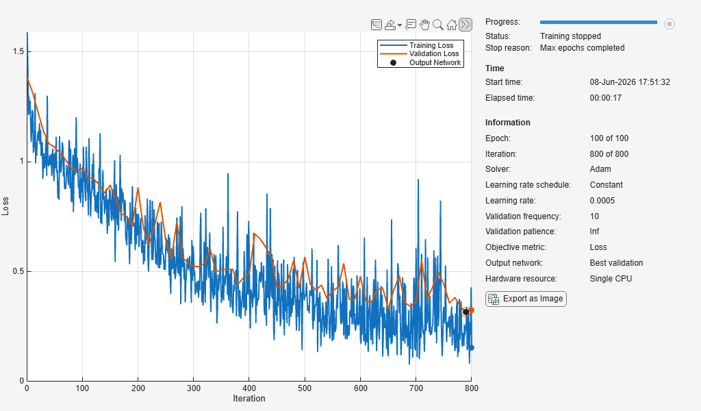
Validation accuracy: 93.7%

Confusion Matrix (Validation):
    23     1     0     0
     1    22     1     0
     1     1    21     1
     0     0     0    23

  Normal accuracy: 95.8%
  Mild accuracy: 91.7%
  Moderate accuracy: 87.5%
  Severe accuracy: 100.0%
The trained network achieves 93.7% validation accuracy, with strongest performance on the Severe and Normal classes. Most misclassifications occur between adjacent severity levels, where clinical boundaries naturally overlap.
Test Trained Classifier
Apply the trained 1D-CNN to the test data and compute the classification accuracy. Misclassifications are typically concentrated between adjacent severity levels where clinical grades genuinely overlap.
numFeatures = size(testFeatures,2);
XTest = reshape(testFeatures',[numFeatures,1,1,size(testFeatures,1)]);

severityNames = {'Normal','Mild','Moderate','Severe'};
YTestTrue = categorical(arrayfun(@(x) severityNames{x+1}, ...
    testWindowLabels,UniformOutput=false),severityNames);
scores = minibatchpredict(trainedNet,XTest);
YTestPred = scores2label(scores,categories(YTestTrue));

testAccuracy = sum(YTestPred == YTestTrue) / numel(YTestTrue) * 100;
fprintf("Classification accuracy: %.1f%%\n",testAccuracy);
Classification accuracy: 93.7%
Display the confusion matrix to evaluate per-class performance.
confusionchart(YTestTrue,YTestPred,Title="1D-CNN Severity Classification", ...
    ColumnSummary="column-normalized",RowSummary="row-normalized");
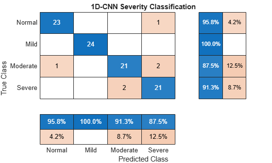
The test accuracy matches the validation result, confirming that the model generalizes well and is suitable for driving the adaptive stimulation controller.
Simulate Adaptive DBS Controller
The ultimate goal is to implement the classification model in an adaptive DBS controller. The controller collects patient LFPs in real-time, classifies symptom severity, and applies appropriate stimulation. Specifically, the controller triggers stimulation when beta-power exceeds a threshold and scales amplitude with predicted severity. For this example, you simulate the controller's behavior on recorded data by combining the training, validation, and test features into one data set.
allFeatures = [trainFeatures;valFeatures;testFeatures];
allLabels = [trainWindowLabels;valWindowLabels;testWindowLabels];
Classify the combined features using the trained network and extract the beta-power for each window.
numAllFeatures = size(allFeatures,2);
XAll = reshape(allFeatures',[numAllFeatures,1,1,size(allFeatures,1)]);
scores = minibatchpredict(trainedNet,XAll);
allPredictions = scores2label(scores,categories(YTestTrue));
betaPower = allFeatures(:,1);
The adaptiveDbsController function provided with this example triggers stimulation when beta-power exceeds a threshold, scales the stimulation amplitude with predicted severity, and ramps gradually to prevent side effects.
controllerParams.windowSec = windowLength;
controllerParams.fs = fs;
stimResults = adaptiveDbsController(allPredictions,betaPower,controllerParams);
Running adaptive DBS controller (477 windows, 1.0s each)...

--- Adaptive DBS Results ---
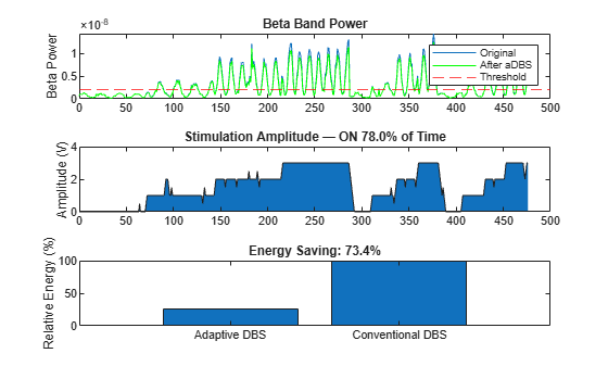
  Time on stimulation: 78.0% (vs 100% conventional)
  Average amplitude when ON: 1.96 V
  Energy saving vs conventional: 73.4%
  Beta threshold: 0.0000
Visualize Stimulation Results
To evaluate stimulation efficiency, visualize the adaptive DBS controller output. The beta-power plot shows the original and suppressed signals, with a threshold line at 20% above median beta-power. The stimulation amplitude plot shows when and how strongly the controller stimulates. Amplitude scales with predicted severity. The controller is active for Mild or higher and inactive for Normal. Points where elevated beta-power coincides with a Normal prediction indicate a potential classification error. The energy savings plot compares the total energy used by adaptive DBS against conventional continuous stimulation.
numWindows = numel(stimResults.amplitude);
timeAxis = (0:numWindows-1) * stimResults.windowSec;

tiledlayout(3,1)
nexttile
plot(timeAxis,stimResults.betaPower);
hold on
plot(timeAxis,stimResults.betaSuppressed,"g");
yline(stimResults.betaThreshold,"r--");
hold off
ylabel("Beta Power");
legend("Original","After aDBS","Threshold");
title("Beta Band Power");

nexttile
area(timeAxis,stimResults.amplitude);
ylabel("Amplitude (V)");
ylim([0 4]);
title(sprintf("Stimulation Amplitude — ON %.1f%% of Time",stimResults.timeOnStim));

nexttile
bar(categorical(["Conventional DBS","Adaptive DBS"]),[100,100-stimResults.energySaving]);
ylabel("Relative Energy (%)");
title(sprintf("Energy Saving: %.1f%%",stimResults.energySaving));
Improve Results
In this example, the adaptive DBS controller reduces energy consumption compared to conventional continuous stimulation while maintaining therapeutic benefit. Improve the system by:
Increasing the amount of training data to improve CNN accuracy
Adjusting the beta-power threshold to fine-tune stimulation sensitivity
Using additional spectral features (for example, phase-amplitude coupling) or longer window lengths for better severity discrimination
Setting separate on and off thresholds for smoother stimulation transitions
Try increasing the overlap fraction from 0.5 to 0.75 in the Extract Beta-Band Features section of this example. Then run the example to observe the impact on classification accuracy and energy savings. When you increase the overlap, the number of training windows nearly doubles. This increase gives the classifier more samples to learn from and can improve classification accuracy.
See Also
Functions
tdmsread|tdmsinfo|tdmsDatastore|trainnet(Deep Learning Toolbox) |trainingOptions(Deep Learning Toolbox) |minibatchpredict(Deep Learning Toolbox) |designfilt(Signal Processing Toolbox) |pwelch(Signal Processing Toolbox) |bandpower(Signal Processing Toolbox)

