Point Cloud Classification Using PointNet Deep Learning
This example shows how to train a PointNet network for point cloud classification.
Point cloud data is acquired by a variety of sensors, such as lidar, radar, and depth cameras. These sensors capture 3-D position information about objects in a scene, which is useful for many applications in autonomous driving and augmented reality. For example, discriminating vehicles from pedestrians is critical for planning the path of an autonomous vehicle. However, training robust classifiers with point cloud data is challenging because of the sparsity of data per object, object occlusions, and sensor noise. Deep learning techniques have been shown to address many of these challenges by learning robust feature representations directly from point cloud data. One of the seminal deep learning techniques for point cloud classification is PointNet [1].
This example trains a PointNet classifier on the Sydney Urban Objects data set created by the University of Sydney [2]. This data set provides a collection of point cloud data acquired from an urban environment using a lidar sensor. The data set has 100 labeled objects from 14 different categories, such as car, pedestrian, and bus.
Load data set
Download and extract the Sydney Urban Objects data set to a temporary directory.
downloadDirectory = tempdir;
datapath = downloadSydneyUrbanObjects(downloadDirectory);
Load the downloaded training and validation data set using the loadSydneyUrbanObjectsData helper function listed at the end of this example. Use the first three data folds for training and the fourth for validation.
foldsTrain = 1:3;
foldsVal = 4;
dsTrain = loadSydneyUrbanObjectsData(datapath,foldsTrain);
dsVal = loadSydneyUrbanObjectsData(datapath,foldsVal);
Read one of the training samples and visualize it using pcshow.
data = read(dsTrain);
ptCloud = data{1,1};
label = data{1,2};

figure
pcshow(ptCloud.Location,[0 1 0],"MarkerSize",40,"VerticalAxisDir","down")
xlabel("X")
ylabel("Y")
zlabel("Z")
title(label)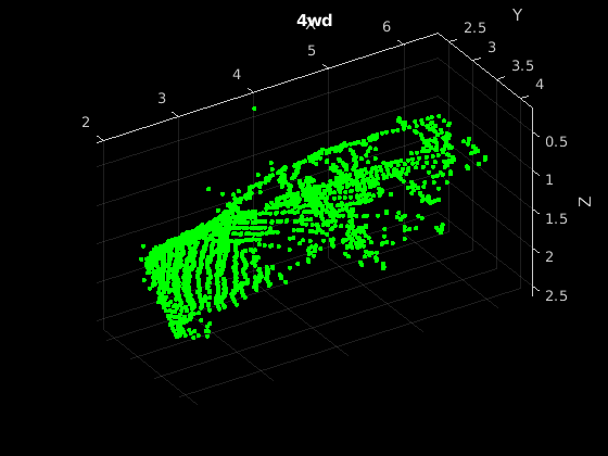
Read the labels and count the number of points assigned to each label to better understand the distribution of labels within the data set.
dsLabelCounts = transform(dsTrain,@(data){data{2} data{1}.Count});
labelCounts = readall(dsLabelCounts);
labels = vertcat(labelCounts{:,1});
counts = vertcat(labelCounts{:,2});
Next, use a histogram to visualize the class distribution.
figure
histogram(labels)
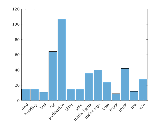
The label histogram shows that the data set is imbalanced and biased towards cars and pedestrians, which can prevent the training of a robust classifier. You can address class imbalance by oversampling the infrequent classes. For the Sydney Urban Objects data set, duplicating files corresponding to the infrequent classes is a simple method to address the class imbalance.
Group the files by label, count the number of observations per class, and use the randReplicateFiles helper function, listed at the end of this example, to randomly oversample the files to the desired number of observations per class.
rng(0)
[G,classes] = findgroups(labels);
numObservations = splitapply(@numel,labels,G);
desiredNumObservationsPerClass = max(numObservations);
files = splitapply(@(x){randReplicateFiles(x,desiredNumObservationsPerClass)},dsTrain.Files,G);
files = vertcat(files{:});
dsTrain.Files = files;
Data Augmentation
Duplicating the files to address class imbalance increases the likelihood of overfitting the network because much of the training data is identical. To offset this effect, apply data augmentation to the training data using the transform and augmentPointCloud helper function, which randomly rotates the point cloud, randomly removes points, and randomly jitters points with Gaussian noise.
dsTrain = transform(dsTrain,@augmentPointCloud);
Preview one of the augmented training samples.
data = preview(dsTrain);
ptCloud = data{1,1};
label = data{1,2};

figure
pcshow(ptCloud.Location,[0 1 0],"MarkerSize",40,"VerticalAxisDir","down")
xlabel("X")
ylabel("Y")
zlabel("Z")
title(label)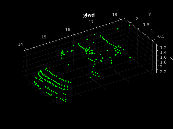
Note that because the data for measuring the performance of the trained network must be representative of the original data set, data augmentation is not applied to validation or test data.
Data Preprocessing
Two preprocessing steps are required to prepare the point cloud data for training and prediction.
First, to enable batch processing during training, select a fixed number of points from each point cloud. The optimal number of points depends on the data set and the number of points required to accurately capture the shape of the object. To help select the appropriate number of points, compute the minimum, maximum, and mean number of points per class.
minPointCount = splitapply(@min,counts,G);
maxPointCount = splitapply(@max,counts,G);
meanPointCount = splitapply(@(x)round(mean(x)),counts,G);

stats = table(classes,numObservations,minPointCount,maxPointCount,meanPointCount)
stats=14×5 table
       classes        numObservations    minPointCount    maxPointCount    meanPointCount
    ______________    _______________    _____________    _____________    ______________

    4wd                      15               140              1955              751
    building                 15               193              8455             2708
    bus                      11               126             11767             2190
    car                      64                52              2377              528
    pedestrian              107                20               297              110
    pillar                   15                80               751              357
    pole                     15                13               253               90
    traffic lights           36                38               352              161
    traffic sign             40                18               736              126
    tree                     24                53              2953              470
    truck                     9               445              3013             1376
    trunk                    42                32               766              241
    ute                      12                90              1380              580
    van                      28                91              5809             1125
Because of the large amount of intra-class and inter-class variability in the number of points per class, choosing a value that fits all classes is difficult. One heuristic is to choose enough points to adequately capture the shape of the objects while not increasing the computational cost by processing too many points. A value of 1024 provides a good tradeoff between these two facets. You can also select the optimal number of points based on empirical analysis. However, that is beyond the scope of this example. Use the transform function to select 1024 points in the training and validation sets.
numPoints = 1024;
dsTrain = transform(dsTrain,@(data)selectPoints(data,numPoints));
dsVal = transform(dsVal,@(data)selectPoints(data,numPoints));
The last preprocessing step is to normalize the point cloud data between 0 and 1 to account for large differences in the range of data values. For example, objects closer to the lidar sensor have smaller values compared to objects that are further away. These differences can hinder the convergence of the network during training. Use transform to normalize the point cloud data in the training and validation sets.
dsTrain = transform(dsTrain,@preprocessPointCloud);
dsVal = transform(dsVal,@preprocessPointCloud);
Preview the augmented and preprocessed training data.
data = preview(dsTrain);
figure
pcshow(data{1,1},[0 1 0],"MarkerSize",40,"VerticalAxisDir","down");
xlabel("X")
ylabel("Y")
zlabel("Z")
title(data{1,2})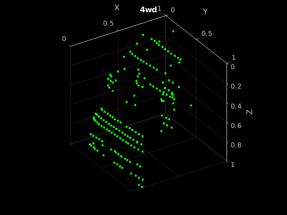
Define PointNet Model
The PointNet classification model consists of two components. The first component is a point cloud encoder that learns to encode sparse point cloud data into a dense feature vector. The second component is a classifier that predicts the categorical class of each encoded point cloud.
The PointNet encoder model is further composed of four models followed by a max operation.
Input transform model
Shared MLP model
Feature transform model
Shared MLP model
The shared MLP model is implemented using a series of convolution, batch normalization, and ReLU operations. The convolution operation is configured such that the weights are shared across the input point cloud. The transform model is composed of a shared MLP and a learnable transform matrix that is applied to each point cloud. The shared MLP and the max operation make the PointNet encoder invariant to the order in which the points are processed, while the transform model provides invariance to orientation changes.
Define PointNet Encoder Model Parameters
The shared MLP and transform models are parameterized by the number of input channels and the hidden channel sizes. The values chosen in this example are selected by tuning these hyperparameters on the Sydney Urban Objects data set. Note that if you want to apply PointNet to a different data set, you must perform additional hyperparameter tuning.
Set the input transform model input channel size to three and the hidden channel sizes to 64, 128, and 256 and use the initializeTransform helper function, listed at the end of this example, to initialize the model parameters.
inputChannelSize = 3;
hiddenChannelSize1 = [64,128];
hiddenChannelSize2 = 256;
[parameters.InputTransform, state.InputTransform] = initializeTransform(inputChannelSize,hiddenChannelSize1,hiddenChannelSize2);
Set the first shared MLP model input channel size to three and the hidden channel size to 64 and use the initializeSharedMLP helper function, listed at the end of this example, to initialize the model parameters.
inputChannelSize = 3;
hiddenChannelSize = [64 64];
[parameters.SharedMLP1,state.SharedMLP1] = initializeSharedMLP(inputChannelSize,hiddenChannelSize);
Set the feature transformation model input channel size to 64 and hidden channel sizes to 64, 128, and 256 and use the initializeTransform helper function, listed at the end of this example, to initialize the model parameters.
inputChannelSize = 64;
hiddenChannelSize1 = [64,128];
hiddenChannelSize2 = 256;
[parameters.FeatureTransform, state.FeatureTransform] = initializeTransform(inputChannelSize,hiddenChannelSize,hiddenChannelSize2);
Set the second shared MLP model input channel size to 64 and the hidden channel size to 64 and use the initializeSharedMLP function, listed at the end of this example, to initialize the model parameters.
inputChannelSize = 64;
hiddenChannelSize = 64;
[parameters.SharedMLP2,state.SharedMLP2] = initializeSharedMLP(inputChannelSize,hiddenChannelSize);
Define PointNet Classifier Model Parameters
The PointNet classifier model consists of a shared MLP, a fully connected operation, and a softmax activation. Set the classifier model input size to 64 and the hidden channel size to 512 and 256 and use the initalizeClassifier helper function, listed at the end of this example, to initialize the model parameters.
inputChannelSize = 64;
hiddenChannelSize = [512,256];
numClasses = numel(classes);
[parameters.ClassificationMLP, state.ClassificationMLP] = initializeClassificationMLP(inputChannelSize,hiddenChannelSize,numClasses);
Define PointNet Function
Create the function pointnetClassifier, listed in the Model Function section at the end of the example, to compute the outputs of the PointNet model. The function model takes as input the point cloud data, the learnable model parameters, the model state, and a flag that specifies whether the model returns outputs for training or prediction. The network returns the predictions for classifying the input point cloud.
Define Model Gradients Function
Create the function modelGradients, listed in the Model Gradients Function section of the example, that takes as input the model parameters, the model state, and a mini-batch of input data, and returns the gradients of the loss with respect to the learnable parameters in the models and the corresponding loss.
Specify Training Options
Train for 10 epochs and load data in batches of 128. Set the initial learning rate to 0.002 and the L2 regularization factor to 0.01.
numEpochs = 10;
learnRate = 0.002;
miniBatchSize = 128;
l2Regularization = 0.01;
learnRateDropPeriod = 15;
learnRateDropFactor = 0.5;
Initialize the options for Adam optimization.
gradientDecayFactor = 0.9;
squaredGradientDecayFactor = 0.999;
Train PointNet
Train the model using a custom training loop.
Shuffle the data at the beginning of training.
For each iteration:
Read a batch of data.
Evaluate the model gradients.
Apply L2 weight regularization.
Use
adamupdateto update the model parameters.Update the training progress plot.
At the end of each epoch, evaluate the model against the validation data set and collect confusion metrics to measure classification accuracy as training progresses.
After completing learnRateDropPeriod epochs, reduce the learning rate by a factor of learnRateDropFactor.
Initialize the moving average of the parameter gradients and the element-wise squares of the gradients used by the Adam optimizer.
avgGradients = [];
avgSquaredGradients = [];
Train the model if doTraining is true. Otherwise, load a pretrained network.
Note that training was verified on an NVIDIA Titan X with 12 GB of GPU memory. If your GPU has less memory, you may run out of memory during training. If this happens, lower the miniBatchSize. Training this network takes about 5 minutes. Depending on your GPU hardware, it can take longer.
doTraining = false;

if doTraining

    % Create a minibatchqueue to batch data from training and validation
    % datastores. Use the batchData function, listed at the end of the
    % example, to batch the point cloud data and one-hot encode the label
    % data.
    numOutputsFromDSRead = 2;
    mbqTrain = minibatchqueue(dsTrain,numOutputsFromDSRead,...
        "MiniBatchSize", miniBatchSize,...
        "MiniBatchFcn",@batchData,...
        "MiniBatchFormat",["SCSB" "BC"]);

    mbqVal = minibatchqueue(dsVal,numOutputsFromDSRead,...
        "MiniBatchSize", miniBatchSize,...
        "MiniBatchFcn",@batchData,...
        "MiniBatchFormat",["SCSB" "BC"]);

    % Use the configureTrainingProgressPlot function, listed at the end of the
    % example, to initialize the training progress plot to display the training
    % loss, training accuracy, and validation accuracy.
    [lossPlotter, trainAccPlotter,valAccPlotter] = initializeTrainingProgressPlot;

    numClasses = numel(classes);
    iteration = 0;
    start = tic;
    for epoch = 1:numEpochs

        % Shuffle data every epoch.
        shuffle(mbqTrain);

        % Iterate through data set.
        while hasdata(mbqTrain)
            iteration = iteration + 1;

            % Read next batch of training data.
            [XTrain, YTrain] = next(mbqTrain);

            % Evaluate the model gradients and loss using dlfeval and the
            % modelGradients function.
            [gradients, loss, state, acc] = dlfeval(@modelGradients,XTrain,YTrain,parameters,state);

            % L2 regularization.
            gradients = dlupdate(@(g,p) g + l2Regularization*p,gradients,parameters);

            % Update the network parameters using the Adam optimizer.
            [parameters, avgGradients, avgSquaredGradients] = adamupdate(parameters, gradients, ...
                avgGradients, avgSquaredGradients, iteration,...
                learnRate,gradientDecayFactor, squaredGradientDecayFactor);

            % Update the training progress.
            D = duration(0,0,toc(start),"Format","hh:mm:ss");
            title(lossPlotter.Parent,"Epoch: " + epoch + ", Elapsed: " + string(D))
            addpoints(lossPlotter,iteration,double(gather(extractdata(loss))))
            addpoints(trainAccPlotter,iteration,acc);
            drawnow
        end

        % Evaluate the model on validation data.
        cmat = sparse(numClasses,numClasses);
        while hasdata(mbqVal)

            % Read next batch of validation data.
            [XVal, YVal] = next(mbqVal);

            % Compute label predictions.
            isTraining = false;
            YPred = pointnetClassifier(XVal,parameters,state,isTraining);

            % Choose prediction with highest score as the class label for
            % XTest.
            [~,YValLabel] = max(YVal,[],1);
            [~,YPredLabel] = max(YPred,[],1);

            % Collect confusion metrics.
            cmat = aggreateConfusionMetric(cmat,YValLabel,YPredLabel);
        end

        % Update training progress plot with average classification accuracy.
        acc = sum(diag(cmat))./sum(cmat,"all");
        addpoints(valAccPlotter,iteration,acc);

        % Upate the learning rate.
        if mod(epoch,learnRateDropPeriod) == 0
            learnRate = learnRate * learnRateDropFactor;
        end

        % Reset training and validation data queues.
        reset(mbqTrain);
        reset(mbqVal);
    end

else
    % Download pretrained model parameters, model state, and validation
    % results.
    pretrainedURL = 'https://ssd.mathworks.com/supportfiles/vision/data/pointnetSydneyUrbanObjects.zip';
    pretrainedResults = downloadPretrainedPointNet(pretrainedURL);

    parameters = pretrainedResults.parameters;
    state = pretrainedResults.state;
    cmat = pretrainedResults.cmat;

    % Move model parameters to the GPU if possible and convert to a dlarray.
    parameters = prepareForPrediction(parameters,@(x)dlarray(toDevice(x,canUseGPU)));

    % Move model state to the GPU if possible.
    state = prepareForPrediction(state,@(x)toDevice(x,canUseGPU));
end
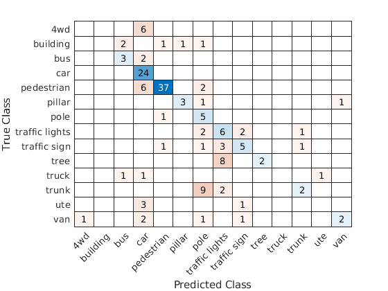
Display the validation confusion matrix.
figure
chart = confusionchart(cmat,classes);
Compute the mean training and validation accuracy.
acc = sum(diag(cmat))./sum(cmat,"all")acc = 0.5742
Due to the limited number of training samples in the Sydney Urban Objects data set, increasing the validation accuracy beyond 60% is challenging. The model easily overfits the training data in the absence of the augmentation defined in the augmentPointCloudData helper function. To improve the robustness of the PointNet classifier, additional training is required.
Classify Point Cloud Data Using PointNet
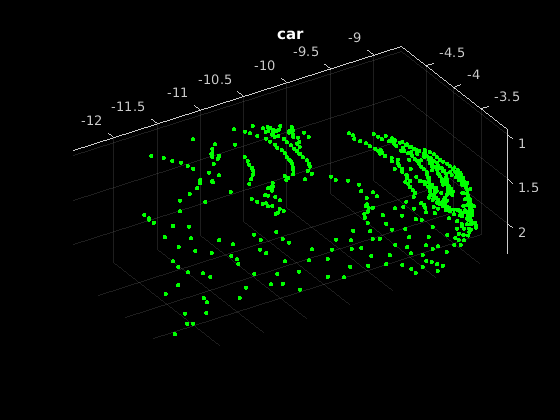
Load point cloud data with pcread, preprocess the point cloud using the same function used during training, and convert the result to a dlarray.
ptCloud = pcread("car.pcd");
X = preprocessPointCloud(ptCloud);
dlX = dlarray(X{1},"SCSB");
Predict point cloud labels with the pointnetClassifier model function.
YPred = pointnetClassifier(dlX,parameters,state,false);
[~,classIdx] = max(YPred,[],1);
Display the point cloud and the predicted label with the highest score.
figure
pcshow(ptCloud.Location,[0 1 0],"MarkerSize",40,"VerticalAxisDir","down")
title(classes(classIdx))
Model Gradients Function
The modelGradients function takes as input a mini-batch of data dlX, the corresponding target dlY, and the learnable parameters, and returns the gradients of the loss with respect to the learnable parameters and the corresponding loss. The loss includes a regularization term designed to ensure the feature transformation matrix predicted by the PointNet encoder is approximately orthogonal. To compute the gradients, evaluate the modelGradients function using the dlfeval function in the training loop.
function [gradients, loss, state, acc] = modelGradients(X,Y,parameters,state)

% Execute the model function.
isTraining = true;
[YPred,state,dlT] = pointnetClassifier(X,parameters,state,isTraining);

% Add regularization term to ensure feature transform matrix is
% approximately orthogonal.
K = size(dlT,1);
B = size(dlT, 4);
I = repelem(eye(K),1,1,1,B);
dlI = dlarray(I,"SSCB");
treg = mse(dlI,pagemtimes(dlT,permute(dlT,[2 1 3 4])));
factor = 0.001;

% Compute the loss.
loss = crossentropy(YPred,Y) + factor*treg;

% Compute the parameter gradients with respect to the loss.
gradients = dlgradient(loss, parameters);

% Compute training accuracy metric.
[~,YTest] = max(Y,[],1);
[~,YPred] = max(YPred,[],1);
acc = gather(extractdata(sum(YTest == YPred)./numel(YTest)));

end
PointNet Classifier Function
The pointnetClassifier function takes as input the point cloud data dlX, the learnable model parameters, the model state, and the flag isTraining, which specifies whether the model returns outputs for training or prediction. Then, the function invokes the PointNet encoder and a multilayer perceptron to extract classification features. During training, dropout is applied after each perceptron operation. After the last perceptron, a fullyconnect operation maps the classification features to the number of classes and a softmax activation is used to normalize the output into a probability distribution of labels. The probability distribution, the updated model state, and the feature transformation matrix predicted by the PointNet encoder are returned as outputs.
function [dlY,state,dlT] = pointnetClassifier(dlX,parameters,state,isTraining)

% Invoke the PointNet encoder.
[dlY,state,dlT] = pointnetEncoder(dlX,parameters,state,isTraining);

% Invoke the classifier.
p = parameters.ClassificationMLP.Perceptron;
s = state.ClassificationMLP.Perceptron;
for k = 1:numel(p)

    [dlY, s(k)] = perceptron(dlY,p(k),s(k),isTraining);

    % If training, apply inverted dropout with a probability of 0.3.
    if isTraining
        probability = 0.3;
        dropoutScaleFactor = 1 - probability;
        dropoutMask = ( rand(size(dlY), "like", dlY) > probability ) / dropoutScaleFactor;
        dlY = dlY.*dropoutMask;
    end

end
state.ClassificationMLP.Perceptron = s;

% Apply final fully connected and softmax operations.
weights = parameters.ClassificationMLP.FC.Weights;
bias = parameters.ClassificationMLP.FC.Bias;
dlY = fullyconnect(dlY,weights,bias);
dlY = softmax(dlY);
end
PointNet Encoder Function
The pointnetEncoder function processes the input dlX using an input transform, a shared MLP, a feature transform, a second shared MLP, and a max operation, and returns the result of the max operation.
function [dlY,state,T] = pointnetEncoder(dlX,parameters,state,isTraining)
% Input transform.
[dlY,state.InputTransform] = dataTransform(dlX,parameters.InputTransform,state.InputTransform,isTraining);

% Shared MLP.
[dlY,state.SharedMLP1.Perceptron] = sharedMLP(dlY,parameters.SharedMLP1.Perceptron,state.SharedMLP1.Perceptron,isTraining);

% Feature transform.
[dlY,state.FeatureTransform,T] = dataTransform(dlY,parameters.FeatureTransform,state.FeatureTransform,isTraining);

% Shared MLP.
[dlY,state.SharedMLP2.Perceptron] = sharedMLP(dlY,parameters.SharedMLP2.Perceptron,state.SharedMLP2.Perceptron,isTraining);

% Max operation.
dlY = max(dlY,[],1);
end
Shared Multilayer Perceptron Function
The shared multilayer perceptron function processes the input dlX using a series of perceptron operations and returns the result of the last perceptron.
function [dlY,state] = sharedMLP(dlX,parameters,state,isTraining)
dlY = dlX;
for k = 1:numel(parameters)
    [dlY, state(k)] = perceptron(dlY,parameters(k),state(k),isTraining);
end
end
Perceptron Function
The perceptron function processes the input dlX using a convolution, a batch normalization, and a relu operation and returns the output of the ReLU operation.
function [dlY,state] = perceptron(dlX,parameters,state,isTraining)
% Convolution.
W = parameters.Conv.Weights;
B = parameters.Conv.Bias;
dlY = dlconv(dlX,W,B);

% Batch normalization. Update batch normalization state when training.
offset = parameters.BatchNorm.Offset;
scale = parameters.BatchNorm.Scale;
trainedMean = state.BatchNorm.TrainedMean;
trainedVariance = state.BatchNorm.TrainedVariance;
if isTraining
    [dlY,trainedMean,trainedVariance] = batchnorm(dlY,offset,scale,trainedMean,trainedVariance);

    % Update state.
    state.BatchNorm.TrainedMean = trainedMean;
    state.BatchNorm.TrainedVariance = trainedVariance;
else
    dlY = batchnorm(dlY,offset,scale,trainedMean,trainedVariance);
end

% ReLU.
dlY = relu(dlY);
end
Data Transform Function
The dataTransform function processes the input dlX using a shared MLP, a max operation, and another shared MLP to predict a transformation matrix T. The transformation matrix is applied to the input dlX using a batched matrix multiply operation. The function returns the result of the batched matrix multiply and the transformation matrix.
function [dlY,state,T] = dataTransform(dlX,parameters,state,isTraining)

% Shared MLP.
[dlY,state.Block1.Perceptron] = sharedMLP(dlX,parameters.Block1.Perceptron,state.Block1.Perceptron,isTraining);

% Max operation.
dlY = max(dlY,[],1);

% Shared MLP.
[dlY,state.Block2.Perceptron] = sharedMLP(dlY,parameters.Block2.Perceptron,state.Block2.Perceptron,isTraining);

% Transform net (T-Net). Apply last fully connected operation as W*X to
% predict tranformation matrix T.
dlY = squeeze(dlY); % N-by-B
T = parameters.Transform * stripdims(dlY); % K^2-by-B

% Reshape T into a square matrix.
K = sqrt(size(T,1));
T = reshape(T,K,K,1,[]); % [K K 1 B]
T = T + eye(K);

% Apply to input dlX using batch matrix multiply.
[C,B] = size(dlX,[3 4]);  % [M 1 K B]
dlX = reshape(dlX,[],C,1,B); % [M K 1 B]
Y = pagemtimes(dlX,T);
dlY = dlarray(Y,"SCSB");
end
Model Parameter Initialization Functions
initializeTransform Function
The initializeTransform function takes as input the channel size and the number of hidden channels for the two shared MLPs, and returns the initialized parameters in a struct. The parameters are initialized using He weight initialization [3].
function [params,state] = initializeTransform(inputChannelSize,block1,block2)
[params.Block1,state.Block1] = initializeSharedMLP(inputChannelSize,block1);
[params.Block2,state.Block2] = initializeSharedMLP(block1(end),block2);

% Parameters for the transform matrix.
params.Transform = dlarray(zeros(inputChannelSize^2,block2(end)));
end
initializeSharedMLP Function
The initializeSharedMLP function takes as input the channel size and the hidden channel size, and returns the initialized parameters in a struct. The parameters are initialized using He weight initialization.
function [params,state] = initializeSharedMLP(inputChannelSize,hiddenChannelSize)
weights = initializeWeightsHe([1 1 inputChannelSize hiddenChannelSize(1)]);
bias = zeros(hiddenChannelSize(1),1,"single");
p.Conv.Weights = dlarray(weights);
p.Conv.Bias = dlarray(bias);

p.BatchNorm.Offset = dlarray(zeros(hiddenChannelSize(1),1,"single"));
p.BatchNorm.Scale = dlarray(ones(hiddenChannelSize(1),1,"single"));

s.BatchNorm.TrainedMean = zeros(hiddenChannelSize(1),1,"single");
s.BatchNorm.TrainedVariance = ones(hiddenChannelSize(1),1,"single");

params.Perceptron(1) = p;
state.Perceptron(1) = s;

for k = 2:numel(hiddenChannelSize)
    weights = initializeWeightsHe([1 1 hiddenChannelSize(k-1) hiddenChannelSize(k)]);
    bias = zeros(hiddenChannelSize(k),1,"single");
    p.Conv.Weights = dlarray(weights);
    p.Conv.Bias = dlarray(bias);

    p.BatchNorm.Offset = dlarray(zeros(hiddenChannelSize(k),1,"single"));
    p.BatchNorm.Scale = dlarray(ones(hiddenChannelSize(k),1,"single"));

    s.BatchNorm.TrainedMean = zeros(hiddenChannelSize(k),1,"single");
    s.BatchNorm.TrainedVariance = ones(hiddenChannelSize(k),1,"single");

    params.Perceptron(k) = p;
    state.Perceptron(k) = s;
end
end
initializeClassificationMLP Function
The initializeClassificationMLP function takes as input the channel size, the hidden channel size, and the number of classes and returns the initialized parameters in a struct. The shared MLP is initialized using He weight initialization and the final fully connected operation is initialized using random Gaussian values.
function [params,state] = initializeClassificationMLP(inputChannelSize,hiddenChannelSize,numClasses)
[params,state] = initializeSharedMLP(inputChannelSize,hiddenChannelSize);

weights = initializeWeightsGaussian([numClasses hiddenChannelSize(end)]);
bias = zeros(numClasses,1,"single");
params.FC.Weights = dlarray(weights);
params.FC.Bias = dlarray(bias);
end
initializeWeightsHe Function
The initializeWeightsHe function initializes parameters using He initialization.
function x = initializeWeightsHe(sz)
fanIn = prod(sz(1:3));
stddev = sqrt(2/fanIn);
x = stddev .* randn(sz);
end
initializeWeightsGaussian Function
The initializeWeightsGaussian function initializes parameters using Gaussian initialization with a standard deviation of 0.01.
function x = initializeWeightsGaussian(sz)
x = randn(sz,"single") .* 0.01;
end
Data Preprocessing Functions
preprocessPointCloudData Function
The preprocessPointCloudData function extracts the X, Y, Z point data from the input data and normalizes the data between 0 and 1. The function returns the normalized X, Y, Z data.
function data = preprocessPointCloud(data)

if ~iscell(data)
    data = {data};
end

numObservations = size(data,1);
for i = 1:numObservations
    % Scale points between 0 and 1.
    xlim = data{i,1}.XLimits;
    ylim = data{i,1}.YLimits;
    zlim = data{i,1}.ZLimits;

    xyzMin = [xlim(1) ylim(1) zlim(1)];
    xyzDiff = [diff(xlim) diff(ylim) diff(zlim)];

    data{i,1} = (data{i,1}.Location - xyzMin) ./ xyzDiff;
end
end
selectPoints Function
The selectPoints function samples the desired number of points. When the point cloud contains more than the desired number of points, the function uses pcdownsample to randomly select points. Otherwise, the function replicates data to produce the desired number of points.
function data = selectPoints(data,numPoints)
% Select the desired number of points by downsampling or replicating
% point cloud data.
numObservations = size(data,1);
for i = 1:numObservations
    ptCloud = data{i,1};
    if ptCloud.Count > numPoints
        percentage = numPoints/ptCloud.Count;
        data{i,1} = pcdownsample(ptCloud,"random",percentage);
    else
        replicationFactor = ceil(numPoints/ptCloud.Count);
        ind = repmat(1:ptCloud.Count,1,replicationFactor);
        data{i,1} = select(ptCloud,ind(1:numPoints));
    end
end
end
Data Augmentation Functions
The augmentPointCloudData function randomly rotates a point cloud about the z-axis, randomly drops 30% of the points, and randomly jitters the point location with Gaussian noise.
function data = augmentPointCloud(data)

numObservations = size(data,1);
for i = 1:numObservations

    ptCloud = data{i,1};

    % Rotate the point cloud about "up axis", which is Z for this data set.
    tform = randomAffine3d(...
        "XReflection", true,...
        "YReflection", true,...
        "Rotation",@randomRotationAboutZ);

    ptCloud = pctransform(ptCloud,tform);

    % Randomly drop out 30% of the points.
    if rand > 0.5
        ptCloud = pcdownsample(ptCloud,'random',0.3);
    end

    if rand > 0.5
        % Jitter the point locations with Gaussian noise with a mean of 0 and
        % a standard deviation of 0.02 by creating a random displacement field.
        D = 0.02 * randn(size(ptCloud.Location));
        ptCloud = pctransform(ptCloud,D);
    end

    data{i,1} = ptCloud;
end
end

function [rotationAxis,theta] = randomRotationAboutZ()
rotationAxis = [0 0 1];
theta = 360*rand;
end
Supporting Functions
aggregateConfusionMetric Function
The aggregateConfusionMetric function incrementally fills a confusion matrix based on the predicted results YPred and the expected results YTest.
function cmat = aggreateConfusionMetric(cmat,YTest,YPred)
YTest = gather(extractdata(YTest));
YPred = gather(extractdata(YPred));
[m,n] = size(cmat);
cmat = cmat + full(sparse(YTest,YPred,1,m,n));
end
initializeTrainingProgressPlot Function
The initializeTrainingProgressPlot function configures two plots for displaying the training loss, training accuracy, and validation accuracy.
function [plotter,trainAccPlotter,valAccPlotter] = initializeTrainingProgressPlot()
% Plot the loss, training accuracy, and validation accuracy.
figure

% Loss plot
subplot(2,1,1)
plotter = animatedline;
xlabel("Iteration")
ylabel("Loss")

% Accuracy plot
subplot(2,1,2)
trainAccPlotter = animatedline('Color','b');
valAccPlotter = animatedline('Color','g');
legend('Training Accuracy','Validation Accuracy','Location','northwest');
xlabel("Iteration")
ylabel("Accuracy")
end
replicateFiles Function
The replicateFiles function randomly oversamples a set of files and returns a set of files with numDesired elements.
function files = randReplicateFiles(files,numDesired)
n = numel(files);
ind = randi(n,numDesired,1);
files = files(ind);
end
downloadSydneyUrbanObjects Function
The downloadSydneyUrbanObjects function downloads the data set and saves it to a temporary directory.
function datapath = downloadSydneyUrbanObjects(dataLoc)

if nargin == 0
    dataLoc = pwd;
end

dataLoc = string(dataLoc);

url = "http://www.acfr.usyd.edu.au/papers/data/";
name = "sydney-urban-objects-dataset.tar.gz";

datapath = fullfile(dataLoc,'sydney-urban-objects-dataset');
if ~exist(datapath,'dir')
    disp('Downloading Sydney Urban Objects data set...');
    untar(url+name,dataLoc);
end

end
loadSydneyUrbanObjectsData Function
The loadSydneyUrbanObjectsData function creates a datastore for loading point cloud and label data from the Sydney Urban Objects data set.
function ds = loadSydneyUrbanObjectsData(datapath,folds)

if nargin == 0
    return;
end

if nargin < 2
    folds = 1:4;
end

datapath = string(datapath);
path = fullfile(datapath,'objects',filesep);

% Add folds to datastore.
foldNames{1} = importdata(fullfile(datapath,'folds','fold0.txt'));
foldNames{2} = importdata(fullfile(datapath,'folds','fold1.txt'));
foldNames{3} = importdata(fullfile(datapath,'folds','fold2.txt'));
foldNames{4} = importdata(fullfile(datapath,'folds','fold3.txt'));
names = foldNames(folds);
names = vertcat(names{:});

fullFilenames = append(path,names);
ds = fileDatastore(fullFilenames,'ReadFcn',@extractTrainingData,'FileExtensions','.bin');
end
batchData Function
The batchData function collates data into batches and moves data to the GPU for processing.
function [X,Y] = batchData(ptCloud,labels)
X = cat(4,ptCloud{:});
labels = cat(1,labels{:});
Y = onehotencode(labels,2);
end
extractTrainingData Function
The extractTrainingData function extracts point cloud and label data from the Sydney Urban Objects data set.
function dataOut = extractTrainingData(fname)

[pointData,intensity] = readbin(fname);

[~,name] = fileparts(fname);
name = string(name);
name = extractBefore(name,'.');
name = replace(name,'_',' ');

labelNames = ["4wd","building","bus","car","pedestrian","pillar",...
    "pole","traffic lights","traffic sign","tree","truck","trunk","ute","van"];

label = categorical(name,labelNames);

dataOut = {pointCloud(pointData,'Intensity',intensity),label};

end
readbin Function
The readbin function reads the point cloud data from Sydney Urban Object binary files.
function [pointData,intensity] = readbin(fname)
% readbin Read point and intensity data from Sydney Urban Object binary
% files.

% names = ['t','intensity','id',...
%          'x','y','z',...
%          'azimuth','range','pid']
%
% formats = ['int64', 'uint8', 'uint8',...
%            'float32', 'float32', 'float32',...
%            'float32', 'float32', 'int32']

fid = fopen(fname, 'r');
c = onCleanup(@() fclose(fid));

fseek(fid,10,-1); % Move to the first X point location 10 bytes from beginning
X = fread(fid,inf,'single',30);
fseek(fid,14,-1);
Y = fread(fid,inf,'single',30);
fseek(fid,18,-1);
Z = fread(fid,inf,'single',30);

fseek(fid,8,-1);
intensity = fread(fid,inf,'uint8',33);

pointData = [X,Y,Z];
end
downloadPretrainedPointNet Function
The downloadPretrainedPointNet function downloads a pretrained pointnet model.
function data = downloadPretrainedPointNet(pretrainedURL)
% Download and load a pretrained pointnet model.
if ~exist('pointnetSydneyUrbanObjects.mat', 'file')
    if ~exist('pointnetSydneyUrbanObjects.zip', 'file')
        disp('Downloading pretrained detector (5 MB)...');
        websave('pointnetSydneyUrbanObjects.zip', pretrainedURL);
    end
    unzip('pointnetSydneyUrbanObjects.zip');
end
data = load("pointnetSydneyUrbanObjects.mat");
end
prepareForPrediction Function
The prepareForPrediction function is used to apply a user-defined function to nested structure data. It is a used to move model parameter and state data to the GPU.
function p = prepareForPrediction(p,fcn)

for i = 1:numel(p)
    p(i) = structfun(@(x)invoke(fcn,x),p(i),'UniformOutput',0);
end

    function data = invoke(fcn,data)
        if isstruct(data)
            data = prepareForPrediction(data,fcn);
        else
            data = fcn(data);
        end
    end
end

% Move data to the GPU.
function x = toDevice(x,useGPU)
if useGPU
    x = gpuArray(x);
end
end
References
[1] Charles, R. Qi, Hao Su, Mo Kaichun, and Leonidas J. Guibas. “PointNet: Deep Learning on Point Sets for 3D Classification and Segmentation.” In 2017 IEEE Conference on Computer Vision and Pattern Recognition (CVPR), 77–85. Honolulu, HI: IEEE, 2017. https://doi.org/10.1109/CVPR.2017.16.
[2] de Deuge, Mark, Alastair Quadras, Calvin Hung, and Bertrand Douillard. "Unsupervised Feature Learning for Classification of Outdoor 3D Scans." In Australasian Conference on Robotics and Automation 2013 (ACRA 13). Sydney, Australia: ACRA, 2013.
[3] He, Kaiming, Xiangyu Zhang, Shaoqing Ren, and Jian Sun. “Delving Deep into Rectifiers: Surpassing Human-Level Performance on ImageNet Classification.” In 2015 IEEE International Conference on Computer Vision (ICCV), 1026–34. Santiago, Chile: IEEE, 2015. https://doi.org/10.1109/ICCV.2015.123.
Related Topics
- Getting Started with Point Clouds Using Deep Learning (Computer Vision Toolbox)
- Define Custom Training Loops, Loss Functions, and Networks
- Specify Training Options in Custom Training Loop
- Train Network Using Custom Training Loop
- List of Deep Learning Layers
- Deep Learning Tips and Tricks
- Automatic Differentiation Background
