混合整数均值-方差投资组合优化问题

此示例说明如何求解具有选定资产数量或条件（半连续）边界约束的均值方差投资组合优化问题。若要求解此问题，您可以使用 Portfolio 对象以及不同的混合整数非线性规划 (MINLP) 求解器。

均值-方差投资组合

加载 CAPMuniverse.mat 中的收益数据。然后，使用默认约束创建一个权重总和为 1 的纯多头投资组合均值方差 Portfolio 对象。对于此示例，您可以将权重 $X$ 的可行域定义为

$X = {x | \sum_{i = 1}^{n} x_{i} = 1, x_{i} \geq 0} .$

% Load data
load CAPMuniverse.mat

% Create a mean-variance Portfolio object with default constraints
p = Portfolio(AssetList=Assets(1:12));
p = estimateAssetMoments(p,Data(:,1:12));
p = setDefaultConstraints(p);

通过设置条件（半连续）边界来包含此场景的二元变量。条件边界是指 $x_{i} = 0$ 或 $x_{i} \geq ℓ_{i}$ 这样的边界。在此示例中，所有资产的边界为 $ℓ_{i} = 0.1$ 。

% Set conditional bounds
condLB = 0.1;
condUB = 0.5;
p = setBounds(p,condLB,condUB,BoundType="conditional");

使用 estimateFrontier 估计有效边界上的一组投资组合。有效边界是一条曲线，该曲线显示帕累托最优投资组合实现的收益和风险之间的平衡。对于给定的收益水平，有效边界上的投资组合是指在保持期望收益的同时将风险降至最低的投资组合。与之相对，对于给定的风险水平，有效边界上的投资组合是指在保持预期风险水平的同时最大化收益的投资组合。

% Compute efficient frontier
pwgt = estimateFrontier(p)

pwgt = 12×10

         0         0    0.1000    0.1253    0.1745    0.2236    0.2715    0.3327    0.4111    0.5000
         0         0         0         0         0         0         0         0         0         0
         0         0         0         0         0         0         0         0         0         0
    0.1350         0         0         0         0         0         0         0         0         0
         0         0         0         0         0         0         0         0         0         0
    0.1000    0.1450    0.1406    0.1910    0.2344    0.2778    0.3200    0.3726    0.4415    0.5000
    0.1000    0.1609    0.1642    0.2121    0.2415    0.2709    0.3085    0.2947    0.1474         0
    0.2354    0.1875    0.1290         0         0         0         0         0         0         0
         0         0         0         0         0         0         0         0         0         0
    0.4296    0.4066    0.3662    0.3717    0.2496    0.1277         0         0         0         0
      ⋮

% Compute risk and returns of the portfolios on the efficient frontier
[rsk,ret] = estimatePortMoments(p,pwgt)

使用 plotFrontier 根据边界估计值绘制权重。生成的曲线呈分段凹形，凹区间之间有垂直跳跃（不连续性）。

% Plot efficient frontier
plotFrontier(p,pwgt)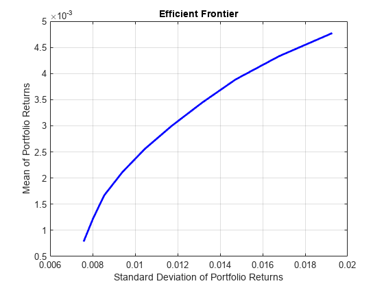

更改 MINLP 求解器

在上一部分，您使用了 estimateFrontier 的默认求解器。但其实您可以使用 setSolverMINLP 支持的下面三种算法中的任意一种来求解混合整数投资组合问题：OuterApproximation、ExtendedCP 和 TrustRegionCP。此外，OuterApproximation 算法在求解 Portfolo 问题时还接受一个额外的名称-值参量 (ExtendedFormulation)，可以重新表述问题的二次函数形式，从而能够在扩展空间中进行处理，这通常会减少计算时间。包括 OuterApproximation 算法的扩展公式变体在内的所有算法，都会在数值精度范围内返回相同的值。可用的求解器包括：

OuterApproximation - 默认算法，该算法非常稳健，通常比 ExtenedCP 速度更快
OuterApproximation，其中 ExtendedFormulation 设置为 true - 一种稳健的算法，通常比其他算法更快，但仅支持求解 Portfolio 对象问题
ExtendedCP - 该求解器稳健性最佳，但通常速度最慢
TrustRegionCP - 该算法速度最快，但稳健性较差，可能提供次优解

有关混合整数投资组合问题求解器的详细信息，请参阅Choose MINLP Solvers for Portfolio Problems。

若要更改 MINLP 求解器，请使用 setSolverMINLP。

% Select the extended formulation version of 'OuterApproximation'
p_EOA = setSolverMINLP(p,'OuterApproximation',...
    ExtendedFormulation=true);
pwgt_EOA = estimateFrontier(p_EOA);
[rskEOA,retEOA] = estimatePortMoments(p_EOA,pwgt_EOA);

% Select 'TrustRegionCP' as solver
p_TR = setSolverMINLP(p,'TrustRegionCP');
pwgt_TR = estimateFrontier(p_TR);
[rskTR,retTR] = estimatePortMoments(p_TR,pwgt_TR);

% Select 'ExtendedCP' as solver using 'midway' cuts as 'CutGeneration'
p_ECP = setSolverMINLP(p,'ExtendedCP','CutGeneration','midway');
pwgt_ECP = estimateFrontier(p_ECP);
[rskECP,retECP] = estimatePortMoments(p_ECP,pwgt_ECP);

比较使用不同的求解器得到的有效边界上的投资组合收益和风险。它们在数值精度内是相同的，其中绝对误差为 $\leq 10^{- 4}$ 。

retTable = table(ret,retEOA,retTR,retECP,...
    'VariableNames',{'OA','EOA','TR','ECP'})

retTable=10×4 table
        OA           EOA            TR           ECP    
    __________    __________    __________    __________

    0.00078336    0.00078336    0.00078334    0.00078348
     0.0012267     0.0012267     0.0012267     0.0012268
       0.00167       0.00167       0.00167     0.0016701
     0.0021133     0.0021133     0.0021133     0.0021134
     0.0025566     0.0025566     0.0025566     0.0025567
     0.0029999     0.0029999     0.0029999         0.003
     0.0034432     0.0034432     0.0034432     0.0034433
     0.0038865     0.0038865     0.0038865     0.0038866
     0.0043298     0.0043298     0.0043298     0.0043299
     0.0047731     0.0047731     0.0047731     0.0047731

rskTable = table(rsk,rskEOA,rskTR,rskECP,...
    'VariableNames',{'OA','EOA','TR','ECP'})

rskTable=10×4 table
       OA           EOA          TR           ECP   
    _________    _________    _________    _________

    0.0075778    0.0075778    0.0075778    0.0075778
    0.0080234    0.0080234    0.0080235    0.0080236
    0.0085488    0.0085488    0.0085488     0.008549
    0.0094024    0.0094024     0.009405    0.0094025
     0.010456     0.010456     0.010456     0.010456
     0.011727     0.011727     0.011776     0.011728
     0.013155     0.013155     0.013155     0.013155
     0.014729     0.014729     0.014729     0.014729
     0.016764     0.016764     0.016764     0.016764
     0.019273     0.019273     0.019273     0.019273

% Compare risks from the different OuterApproximation formulations
norm(rskTable.OA-rskTable.EOA,Inf) <= 1e-4

ans = logical
   1

另请参阅

estimatePortSharpeRatio | estimateFrontier | estimateFrontierByReturn | estimateFrontierByRisk

详细信息

Choose MINLP Solvers for Portfolio Problems

混合整数均值-方差投资组合优化问题

均值-方差投资组合

更改 MINLP 求解器

另请参阅

相关示例

详细信息

WeChat