Portfolio Optimization Against a Benchmark
This example shows how to perform portfolio optimization using the Portfolio object in Financial Toolbox™.
This example, in particular, demonstrates optimizing a portfolio to maximize the information ratio relative to a market benchmark. Specifically, financial data contained in a table is read into MATLAB® and visualizations (at both daily and annual levels) are performed. A Portfolio object is created with the market data using an active daily return for each asset. Using functions supporting a Portfolio object, the efficient frontier is calculated directly and a customized optimization problem is solved to find the asset allocation with the maximized information ratio.

Import Historical Data Using MATLAB®
Import historical prices for the asset universe and the Dow Jones Industrial Average (DJI) market benchmark. The data is imported into a table from a Microsoft® Excel® spreadsheet using the MATLAB® readtable function.
data = readtable('dowPortfolio.xlsx');
head(data, 10)
Dates DJI AA AIG AXP BA C CAT DD DIS GE GM HD HON HPQ IBM INTC JNJ JPM KO MCD MMM MO MRK MSFT PFE PG T UTX VZ WMT XOM
___________ _____ _____ _____ _____ _____ _____ _____ _____ _____ _____ _____ _____ _____ _____ _____ _____ _____ _____ _____ _____ _____ _____ _____ _____ _____ _____ _____ _____ _____ _____ _____
03-Jan-2006 10847 28.72 68.41 51.53 68.63 45.26 55.86 40.68 24.18 33.6 17.82 39.79 36.14 28.35 80.13 24.57 59.08 37.78 38.98 32.72 75.93 52.27 30.73 26.19 22.16 56.38 22.7 54.94 26.79 44.9 56.64
04-Jan-2006 10880 28.89 68.51 51.03 69.34 44.42 57.29 40.46 23.77 33.56 18.3 39.05 35.99 29.18 80.03 24.9 59.99 37.56 38.91 33.01 75.54 52.65 31.08 26.32 22.88 56.48 22.87 54.61 27.58 44.99 56.74
05-Jan-2006 10882 29.12 68.6 51.57 68.53 44.65 57.29 40.38 24.19 33.47 19.34 38.67 35.97 28.97 80.56 25.25 59.74 37.67 39.1 33.05 74.85 52.52 31.13 26.34 22.9 56.3 22.92 54.41 27.9 44.38 56.45
06-Jan-2006 10959 29.02 68.89 51.75 67.57 44.65 58.43 40.55 24.52 33.7 19.61 38.96 36.53 29.8 82.96 25.28 60.01 37.94 39.47 33.25 75.47 52.95 31.08 26.26 23.16 56.24 23.21 54.58 28.01 44.56 57.57
09-Jan-2006 11012 29.37 68.57 53.04 67.01 44.43 59.49 40.32 24.78 33.61 21.12 39.38 36.23 30.17 81.76 25.44 60.38 38.55 39.66 33.88 75.84 53.11 31.58 26.21 23.16 56.67 23.3 55.2 28.12 44.4 57.54
10-Jan-2006 11012 28.44 69.18 52.88 67.33 44.57 59.25 40.2 25.09 33.43 20.79 40.33 36.17 30.33 82.1 25.1 60.49 38.61 39.7 33.91 75.37 53.04 31.27 26.35 22.77 56.45 23.16 55.24 28.24 44.54 57.99
11-Jan-2006 11043 28.05 69.6 52.59 68.3 44.98 59.28 38.87 25.33 33.66 20.61 41.44 36.19 30.88 82.19 25.12 59.91 38.58 39.72 34.5 75.22 53.31 31.39 26.63 23.06 56.65 23.34 54.41 28.58 45.23 58.38
12-Jan-2006 10962 27.68 69.04 52.6 67.9 45.02 60.13 38.02 25.41 33.25 19.76 41.05 35.77 30.57 81.61 24.96 59.63 37.87 39.5 33.96 74.57 53.23 31.41 26.48 22.9 56.02 23.24 53.9 28.69 44.43 57.77
13-Jan-2006 10960 27.81 68.84 52.5 67.7 44.92 60.24 37.86 25.47 33.35 19.2 40.43 35.85 31.43 81.22 24.78 59.26 37.84 39.37 33.65 74.38 53.29 31.4 26.53 22.99 56.49 23.27 54.1 28.75 44.1 59.06
17-Jan-2006 10896 27.97 67.84 52.03 66.93 44.47 60.85 37.75 25.15 33.2 18.68 40.11 35.56 31.2 81.05 24.52 58.74 37.64 39.11 33.77 73.99 52.85 31.16 26.34 22.63 56.25 23.13 54.41 28.12 43.66 59.61
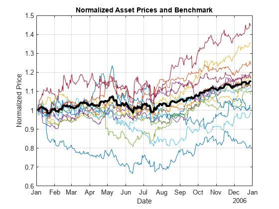
Separate the asset names, asset prices, and DJI benchmark prices from the table. The visualization shows the evolution of all the asset prices normalized to start at unity, that is accumulative returns.
benchPrice = data.DJI;
assetNames = data.Properties.VariableNames(3:2:end); % Use half of the assets for display.
assetPrice = data(:,assetNames).Variables;

assetP = assetPrice./assetPrice(1, :);
benchmarkP = benchPrice / benchPrice(1);

figure;
plot(data.Dates,assetP);
hold on;
plot(data.Dates,benchmarkP,'LineWidth',3,'Color','k');
hold off;
xlabel('Date');
ylabel('Normalized Price');
title('Normalized Asset Prices and Benchmark');
grid on;

The bold line indicates the DJIA market benchmark.
Compute Returns and Risk-Adjusted Returns
Calculate the return series from the price series and compute the asset moments (historical returns and standard deviations). The visualization shows a scatter plot of the risk-return characteristics of all the assets and the DJI market benchmark.
benchReturn = tick2ret(benchPrice);
assetReturn = tick2ret(assetPrice);

benchRetn = mean(benchReturn);
benchRisk =  std(benchReturn);
assetRetn = mean(assetReturn);
assetRisk =  std(assetReturn);
Calculate historical statistics and plot the annual risk-return. Note that the plot is at the annual level, therefore scaling is performed on the daily returns.
scale = 252;

assetRiskR = sqrt(scale) * assetRisk;
benchRiskR = sqrt(scale) * benchRisk;
assetReturnR = scale * assetRetn;
benchReturnR = scale * benchRetn;

figure;
scatter(assetRiskR, assetReturnR, 6, 'm', 'Filled');
hold on
scatter(benchRiskR, benchReturnR, 6, 'g', 'Filled');
for k = 1:length(assetNames)
    text(assetRiskR(k) + 0.005, assetReturnR(k), assetNames{k}, 'FontSize', 8);
end
text(benchRiskR + 0.005, benchReturnR, 'Benchmark', 'Fontsize', 8);
hold off;

xlabel('Risk (Std Dev of Return)');
ylabel('Expected Annual Return');
grid on;

Set Up a Portfolio Optimization
Set up a portfolio optimization problem by populating the object using Portfolio. Because the goal is to optimize portfolio allocation against a benchmark, the active return of each asset is computed and used in the Portfolio object. In this example, the expected returns and covariances of the assets in the portfolio are set to their historical values.
p = Portfolio('AssetList',assetNames);Set up default portfolio constraints (all weights sum to 1, no shorting, and 100% investment in risky assets).
p = setDefaultConstraints(p);
Add asset returns and covariance to the Portfolio object.
activReturn = assetReturn - benchReturn;
pAct = estimateAssetMoments(p,activReturn,'missingdata',false)
pAct =
Portfolio with properties:
BuyCost: []
SellCost: []
RiskFreeRate: []
AssetMean: [15×1 double]
AssetCovar: [15×15 double]
TrackingError: []
TrackingPort: []
Turnover: []
BuyTurnover: []
SellTurnover: []
Name: []
NumAssets: 15
AssetList: {'AA' 'AXP' 'C' 'DD' 'GE' 'HD' 'HPQ' 'INTC' 'JPM' 'MCD' 'MO' 'MSFT' 'PG' 'UTX' 'WMT'}
InitPort: []
AInequality: []
bInequality: []
AEquality: []
bEquality: []
LowerBound: [15×1 double]
UpperBound: []
LowerBudget: 1
UpperBudget: 1
GroupMatrix: []
LowerGroup: []
UpperGroup: []
GroupA: []
GroupB: []
LowerRatio: []
UpperRatio: []
MinNumAssets: []
MaxNumAssets: []
ConditionalBudgetThreshold: []
ConditionalUpperBudget: []
BoundType: [15×1 categorical]
Compute the Efficient Frontier Using the Portfolio Object
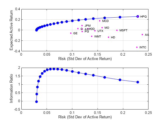
Compute the mean-variance efficient frontier of 20 optimal portfolios. Visualize the frontier over the risk-return characteristics of the individual assets. Furthermore, calculate and visualize the information ratio for each portfolio along the frontier.
pwgtAct = estimateFrontier(pAct, 20); % Estimate the weights.
[portRiskAct, portRetnAct] = estimatePortMoments(pAct, pwgtAct); % Get the risk and return.

% Extract the asset moments and names.
[assetActRetnDaily, assetActCovarDaily] = getAssetMoments(pAct);
assetActRiskDaily = sqrt(diag(assetActCovarDaily));
assetNames = pAct.AssetList;

% Rescale.
assetActRiskAnnual = sqrt(scale) * assetActRiskDaily;
portRiskAnnual  = sqrt(scale) *  portRiskAct;
assetActRetnAnnual = scale * assetActRetnDaily;
portRetnAnnual = scale *  portRetnAct;

figure;
subplot(2,1,1);
plot(portRiskAnnual, portRetnAnnual, 'bo-', 'MarkerFaceColor', 'b');
hold on;

scatter(assetActRiskAnnual, assetActRetnAnnual, 12, 'm', 'Filled');
hold on;
for k = 1:length(assetNames)
    text(assetActRiskAnnual(k) + 0.005, assetActRetnAnnual(k), assetNames{k}, 'FontSize', 8);
end

hold off;

xlabel('Risk (Std Dev of Active Return)');
ylabel('Expected Active Return');
grid on;

subplot(2,1,2);
plot(portRiskAnnual, portRetnAnnual./portRiskAnnual, 'bo-', 'MarkerFaceColor', 'b');
xlabel('Risk (Std Dev of Active Return)');
ylabel('Information Ratio');
grid on;

Perform Information Ratio Maximization
Find the portfolio along the frontier with the maximum information ratio. The information ratio is the ratio of relative return to relative risk (also known as the "tracking error"). Whereas the Sharpe ratio looks at returns relative to a riskless asset, the information ratio is based on returns relative to a risky benchmark, in this case the DJI benchmark. You can compute the information ratio using estimateCustomObjectivePortfolio.
infoRatio = @(x) (pAct.AssetMean'*x)/sqrt(x'*pAct.AssetCovar*x);
optWts = estimateCustomObjectivePortfolio(pAct,infoRatio,...
    ObjectiveSense="maximize");
Get the information ratio, risk, and return for the optimal portfolio.
optInfoRatio = infoRatio(optWts);
[optPortRisk,optPortRetn] = estimatePortMoments(pAct,optWts)
optPortRisk =
0.0040
optPortRetn =
4.8166e-04
Plot the Optimal Portfolio
Verify that the portfolio found is indeed the maximum information-ratio portfolio.
% Rescale.
optPortRiskAnnual = sqrt(scale) * optPortRisk;
optPortReturnAnnual = scale * optPortRetn;

figure;
subplot(2,1,1);

scatter(assetActRiskAnnual, assetActRetnAnnual, 6, 'm', 'Filled');
hold on
for k = 1:length(assetNames)
    text(assetActRiskAnnual(k) + 0.005,assetActRetnAnnual(k),assetNames{k},'FontSize',8);
end
plot(portRiskAnnual,portRetnAnnual,'bo-','MarkerSize',4,'MarkerFaceColor','b');
plot(optPortRiskAnnual,optPortReturnAnnual,'ro-','MarkerFaceColor','r');
hold off;

xlabel('Risk (Std Dev of Active Return)');
ylabel('Expected Active Return');
grid on;

subplot(2,1,2);
plot(portRiskAnnual,portRetnAnnual./portRiskAnnual,'bo-','MarkerSize',4,'MarkerFaceColor','b');
hold on
plot(optPortRiskAnnual,optPortReturnAnnual./optPortRiskAnnual,'ro-','MarkerFaceColor','r');
hold off;

xlabel('Risk (Std Dev of Active Return)');
ylabel('Information Ratio');
title('Information Ratio with Optimal Portfolio');
grid on;

Display the Portfolio Optimization Solution
Display the portfolio optimization solution.
assetIndx = optWts > .001;
results = table(assetNames(assetIndx)', optWts(assetIndx)*100, 'VariableNames',{'Asset', 'Weight'});
disp('Maximum Information Ratio Portfolio:')
Maximum Information Ratio Portfolio:
disp(results)
     Asset      Weight
    ________    _______

    {'AA'  }     1.5389
    {'AXP' }    0.35545
    {'C'   }     9.6533
    {'DD'  }     4.0684
    {'HPQ' }     17.699
    {'JPM' }     21.565
    {'MCD' }     26.736
    {'MO'  }     13.648
    {'MSFT'}     2.6858
    {'UTX' }     2.0509
fprintf('Active return for Max. Info Ratio portfolio is %0.2f%%n', optPortRetn*25200);Active return for Max. Info Ratio portfolio is 12.14%
fprintf('Tracking error for Max. Info Ratio portfolio is %0.2f%%n', optPortRisk*sqrt(252)*100);Tracking error for Max. Info Ratio portfolio is 6.32%
See Also
Portfolio | inforatio | fminbnd
Topics
- Creating the Portfolio Object
- Working with Portfolio Constraints Using Defaults
- Validate the Portfolio Problem for Portfolio Object
- Estimate Efficient Portfolios for Entire Efficient Frontier for Portfolio Object
- Estimate Efficient Frontiers for Portfolio Object
- Postprocessing Results to Set Up Tradable Portfolios
- Portfolio Optimization Examples Using Financial Toolbox
- Portfolio Optimization with Semicontinuous and Cardinality Constraints
- Black-Litterman Portfolio Optimization Using Financial Toolbox
- Portfolio Optimization Using Factor Models
- Portfolio Optimization Using Social Performance Measure
- Diversify Portfolios Using Custom Objective
- Performance Metrics Overview
- Portfolio Object
- Portfolio Optimization Theory
- Portfolio Object Workflow