Using Extreme Value Theory and Copula Fitting to Generate Synthetic Data

Prepare Equity Index Data

Before applying EVT and fitting the data to a copula model, ensure that the observations are approximately independent and identically distributed (iid). To overcome the issues of autocorrelation (dependence on past values) and heteroskedasticity (changing variance over time) that violate the iid assumption, you can use the Autoregressive Integrated Moving Average (ARIMA) and Generalized Autoregressive Conditional Heteroskedasticity (GARCH) models.

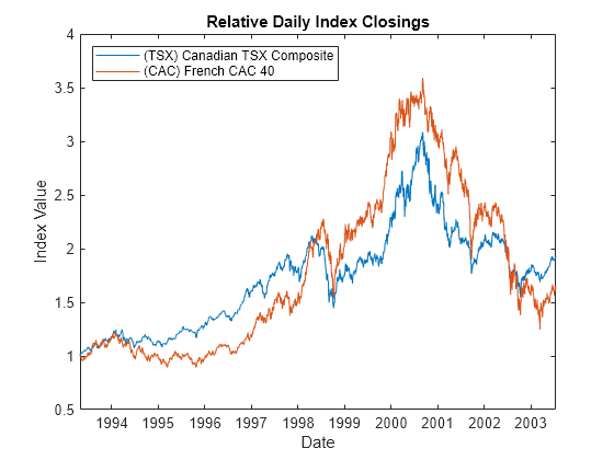
Load the equity index data from the Data_GlobalIdx1 file. The raw data consists of 2665 observations of daily closing values of the Canadian TSX Composite and French CAC 40 indexes spanning the trading dates 27-April-1993 to 14-July-2003.

load Data_GlobalIdx1   % Import daily index closings
Data = Data(:,1:2);
series = string(series(1:2));

Plot these equity indexes to see their relative price movements of these equity indexes.

figure
dates = datetime(dates,'ConvertFrom','datenum');
plot(dates, ret2price(price2ret(Data)))
xlabel('Date')
ylabel('Index Value')
title ('Relative Daily Index Closings')
legend(series, 'Location', 'NorthWest')

Filter Returns for Equity Index

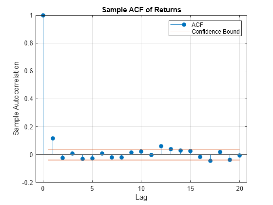
To accurately model the tails of a distribution using a GPD, you must make sure the observations are approximately independent and identically distributed. However, financial return series often deviate from this requirement due to autocorrelation and heteroskedasticity. To see an example of this deviation, use autocorr (Econometrics Toolbox) to analyze the sample autocorrelation function (ACF) of the returns associated with the TSX Composite index. The result indicates the presence of mild serial correlation.

returns = price2ret(Data);    % Logarithmic returns
T       = size(returns,1);    % Number of returns (the historical sample size)

index = 1;
figure
autocorr(returns(:,index))
title('Sample ACF of Returns')

Heteroskedasticity refers to the changing variance of a variable over time. The sample ACF of the squared returns shows the degree of persistence in variance.

figure
autocorr(returns(:,index).^2)
title('Sample ACF of Squared Returns')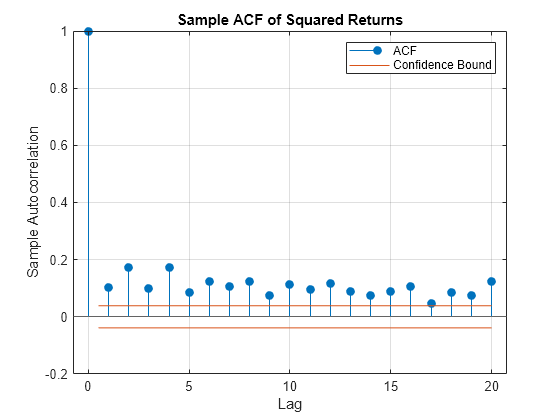

To remove autocorrelation from the equity index return data, you can apply the ARIMA model by using arima (Econometrics Toolbox). ARIMA models are widely used to capture the autocorrelation structure in time series data. By estimating the parameters of the ARIMA model, you can generate residuals that are approximately independent. To address heteroskedasticity in the equity index return data, you can use arima with the Glosten-Jagannathan-Runkle GARCH (GJR) model. GJR models are effective in capturing the time-varying volatility observed in financial return series. By estimating the parameters of the GJR model, you can generate standardized residuals with a constant variance.

Extract the filtered residuals and conditional variances from the returns of the equity index.

model     = arima('AR', NaN, 'Distribution', 't', 'Variance', gjr(1,1));
nIndices  = size(Data,2);        % Number of indices
residuals = NaN(T, nIndices);    % Preallocate storage
variances = NaN(T, nIndices);
fit       = cell(nIndices,1);

options   = optimoptions(@fmincon, 'Display', 'off', ...
    'Diagnostics', 'off', 'Algorithm', 'sqp', 'TolCon', 1e-7);

for i = 1:nIndices
    fit{i} = estimate(model, returns(:,i), 'Display', 'off', 'Options', options);
    [residuals(:,i), variances(:,i)] = infer(fit{i}, returns(:,i));
end

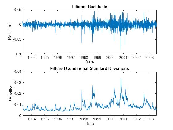
For the TSX Composite index, compare the model residuals and the corresponding conditional standard deviations filtered from the raw returns. The lower graph clearly shows the variation in volatility (heteroskedasticity) of the filtered residuals.

figure
subplot(2,1,1)
plot(dates(2:end), residuals(:,index))
xlabel('Date')
ylabel('Residual')
title ('Filtered Residuals')

subplot(2,1,2)
plot(dates(2:end), sqrt(variances(:,index)))
xlabel('Date')
ylabel('Volatility')
title ('Filtered Conditional Standard Deviations')

To estimate the tails of the cumulative distribution function (CDF) using EVT, you must standardize the residuals by their corresponding conditional standard deviation. These standardized residuals represent a series that is zero-mean, unit-variance, and approximately independent and identically distributed. The EVT estimation of the sample CDF tails is based on this standardized residual series:

residuals = residuals ./ sqrt(variances);

Use autocorr (Econometrics Toolbox) to analyze the autocorrelation functions (ACFs) of the standardized residuals and squared standardized residuals. By comparing these ACFs to the ACFs of the raw returns, you can observe that the standardized residuals exhibit a closer approximation to the iid assumption. The standardized residuals are more suitable for subsequent tail estimation purposes.

figure
autocorr(residuals(:,index))
title('Sample ACF of Standardized Residuals')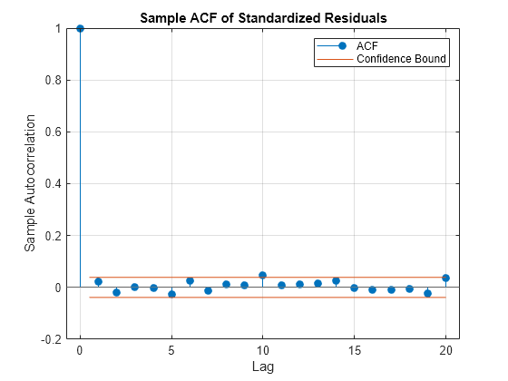

figure
autocorr(residuals(:,index).^2)
title('Sample ACF of Squared Standardized Residuals')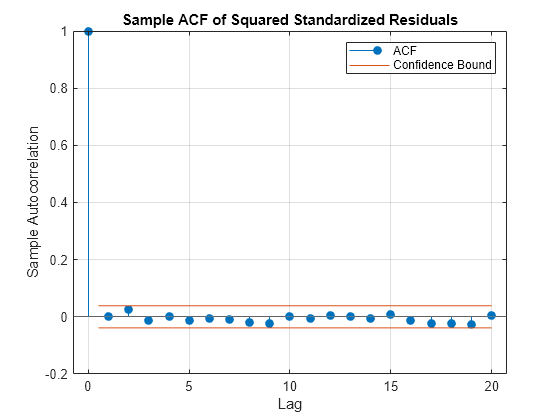

Estimate Semiparametric CDFs

Using the standardized iid residuals from the Filter Returns for Equity Index section, estimate the empirical CDF of each index with a Gaussian kernel. Specifically, estimate the empirical CDF such that the upper and lower thresholds have 10% of the residuals reserved for the tail. Then you can fit the amount that those extreme residuals in the tail fall beyond the associated threshold to a parametric GPD by maximum likelihood.

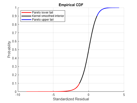
The following code creates an object of type paretotails. The paretotails object encapsulates the estimates of the parametric generalized Pareto (GP) lower tail, the nonparametric kernel-smoothed interior, and the parametric GP upper tail to construct a composite semiparametric CDF for each index. This combination forms a composite semiparametric cumulative distribution function (CDF) for the index.

The paretotails object offers methods to evaluate the CDF and inverse CDF (quantile function). It also provides the ability to query cumulative probabilities and quantiles of the boundaries between each segment of the piecewise distribution.

nPoints      = 200;      % Number of sampled points in each region of the CDF
tailFraction = 0.1;      % Decimal fraction of residuals allocated to each tail

tails = cell(nIndices,1);  % Cell array of Pareto tail objects

for i = 1:nIndices
    tails{i} = paretotails(residuals(:,i), tailFraction, 1 - tailFraction, 'kernel');
end

Having estimated the three distinct regions of the composite semiparametric empirical CDF, you can graphically concatenate and display the result. The lower and upper tail regions, displayed in red and blue, respectively, are suitable for extrapolation, while the kernel-smoothed interior, in black, is suitable for interpolation.

The following code calls the CDF and inverse CDF methods of the paretotails object with different data. Specifically, the referenced methods have access to the fitted state and are now invoked to select and analyze specific regions of the probability curve, acting as a powerful data filtering mechanism.

figure
hold on
grid on

minProbability = cdf(tails{index}, (min(residuals(:,index))));
maxProbability = cdf(tails{index}, (max(residuals(:,index))));

pLowerTail = linspace(minProbability  , tailFraction    , nPoints); % Sample lower tail
pUpperTail = linspace(1 - tailFraction, maxProbability  , nPoints); % Sample upper tail
pInterior  = linspace(tailFraction    , 1 - tailFraction, nPoints); % Sample interior

plot(icdf(tails{index}, pLowerTail), pLowerTail, 'red'  , 'LineWidth', 2)
plot(icdf(tails{index}, pInterior) , pInterior , 'black', 'LineWidth', 2)
plot(icdf(tails{index}, pUpperTail), pUpperTail, 'blue' , 'LineWidth', 2)

xlabel('Standardized Residual')
ylabel('Probability')
title('Empirical CDF')
legend({'Pareto lower tail' 'Kernel smoothed interior' ...
        'Pareto upper tail'}, 'Location', 'NorthWest')

Assess GPD Fit

Examine the GPD fit in more detail.

The CDF of a GPD is parameterized as

for exceedances (y), tail index parameter ($\zeta$), and scale parameter ($\beta$).

To visually assess the GPD fit, plot the empirical CDF of the upper tail exceedances of the residuals along with the CDF fitted by the GPD. Although only 10% of the standardized residuals are used, the fitted distribution closely follows the exceedance data, so the GPD model is an appropriate choice.

figure
[P,Q] = boundary(tails{index});  % Cumulative probabilities & quantiles at boundaries
y     = sort(residuals(residuals(:,index) > Q(2), index) - Q(2)); % Sort exceedances
plot(y, (cdf(tails{index}, y + Q(2)) - P(2))/P(1))
[F,x] = ecdf(y);                 % Empirical CDF
hold on
stairs(x, F, 'r')
grid on

legend('Fitted generalized Pareto CDF','Empirical CDF','Location','SouthEast');
xlabel('Exceedance')
ylabel('Probability')
title('Upper Tail of Standardized Residuals')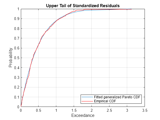

Calibrate t Copula

Given the standardized residuals, you can estimate the scalar degrees of freedom parameter (DoF) and the linear correlation matrix (R) of the t copula using the copulafit function. To transform the residuals, you can use the inverse of the cumulative distribution function (CDF) of the fitted extreme value distribution. This transformation ensures that the residuals follow a uniform distribution, which is a requirement for copula fitting. Then by fitting the t copula to the transformed residuals, you can capture the dependence structure between the equity index returns.

U = zeros(size(residuals));

for i = 1:nIndices
    U(:,i) = cdf(tails{i}, residuals(:,i)); % Transform margin to uniform
end

[R, DoF] = copulafit('t', U, 'Method', 'approximateml'); % Fit the copula

Simulate Index Returns with t Copula

Having fitted the copula, you can generate synthetic equity index return data by sampling from the fitted copula and transforming the samples to standardized residuals by using the inversion of the semiparametric marginal CDF of each index. This process involves extrapolating into the generalized Pareto tails and then interpolating into the smoothed interior. The process ensures that the simulated standardized residuals align with those obtained from the AR(1) + GJR(1,1) filtering process. The simulated standardized residuals are independent in time but exhibit dependence at any given point in time. Each column of the simulated standardized residuals array represents an iid univariate stochastic process when examined individually. However, each row shares the rank correlation induced by the copula.

By simulating the dependent standardized residuals using copularnd, you can create new data that possesses similar statistical properties and dependence structure as the original equity index returns. This new data enables the generation of jointly dependent equity index returns.

The following code simulates 1000 independent random trials of dependent standardized index residuals. These trials are simulated over a period of the same length as the original index data.

s = RandStream.getGlobalStream();
reset(s)

nTrials = 1000;                                  % Number of independent random trials
horizon = size(Data,1);                          % Simulation horizon

Z = zeros(horizon, nTrials, nIndices);            % Standardized residuals array
U = copularnd('t', R, DoF, horizon * nTrials);    % t copula simulation

for j = 1:nIndices
    Z(:,:,j) = reshape(icdf(tails{j}, U(:,j)), horizon, nTrials);
end

Using the simulated standardized residuals as the iid input noise process, you can reintroduce the autocorrelation and heteroskedasticity observed in the original index returns using filter (Econometrics Toolbox).

The filter function accepts user-specified standardized disturbances derived from the copula and simulates multiple paths for a single index model at a time. All sample paths are simulated and stored for each index in succession.

To make the most of the current information, specify the necessary presample model residuals, variances, and returns so that each simulated path evolves from a common initial state.

Y0 = returns(1,:);                    % Presample returns
Z0 = residuals(1,:);                  % Presample standardized residuals
V0 = variances(1,:);                  % Presample variances

simulatedReturns = zeros(horizon, nTrials, nIndices);

for i = 1:nIndices
    simulatedReturns(:,:,i) = filter(fit{i}, Z(:,:,i), ...
                                    'Y0', Y0(i), 'Z0', Z0(i), 'V0', V0(i));
end

Summarize Results

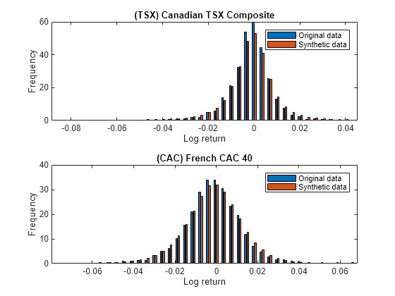
Once the returns of each index are simulated, you can plot the histograms of returns to visually observe the presence of the fat tail phenomenon. By adjusting the bin width or number of bins (nBins) in the histogram, you can control the level of detail and granularity in the representation of the distribution.

tiledlayout(2,1)

for i = 1:nIndices   
    nexttile
    nBins = 40;

    [data1,edge] = histcounts(returns(:,i),nBins,'Normalization','pdf');
    [I1,edge] = histcounts(simulatedReturns(:,:,i),edge,'Normalization','pdf');
    bar(edge(1:end-1),[data1;I1])    
        
    hold('on')    
    
    xlabel('Log return')
    ylabel('Frequency')
    title (series(i))
    legend("Original data", "Synthetic data")
end