Use Deep Learning to Approximate Barrier Option Prices with Heston Model

Barrier Option

The barrier option is an option where the payoff depends on whether the underlying asset crosses the predetermined trigger value (barrier level) during the life of the option. Barrier options are attractive because they are less expensive than the corresponding vanilla options. For more information, see Barrier Option.

Heston Model

The Heston model is an extension of the Black-Scholes model, where the volatility (square root of variance) is no longer assumed to be constant, and the variance follows a stochastic (CIR) process. The Heston model allows modeling the implied volatility smiles observed in the market where options with identical expiration dates show increasing volatility as the options become more in-the-money (ITM) or out-of-the-money (OTM).

The stochastic differential equation is:

where

$\mathit{r}$ — Continuous risk-free rate

${\mathit{S}}_{\mathit{t}}$ — Asset price at time $\mathit{t}$

${\mathit{v}}_{\mathit{t}}$ — Asset price variance at time $\mathit{t}$

${\mathit{v}}_0$ — Initial variance of the asset price at $\mathit{t}=0$

$\theta$ — Long-term variance level

$\kappa$ — Mean reversion speed for the variance

${\sigma }_{\mathit{v}}$ — Volatility of the variance

$\rho$ — Correlation between the Wiener processes ${\mathit{W}}_{\mathit{t}}$ and ${\mathit{W}}_{\mathit{t}}^{\mathit{v}}$

Barrier option prices are usually computed using Monte Carlo simulation in the Heston setting since there is no closed-form solution available. However, a Monte Carlo simulation is computationally expensive, and when pricing instruments for financial markets, pricing speed is crucial. This example demonstrates using a vanilla neural network to speed up the barrier option pricing by learning the results from a Monte Carlo simulation. The neural network provides a highly efficient approximation technique. Although the off-line training is time consuming, the on-line pricing is fast.

Define Parameters

Focusing on a barrier-up, knock-out call option, start by deciding on the ranges for the pricing parameters. Consider a scaled spot price (moneyness) instead of two separate parameters ${\mathit{S}}_0$ (asset spot price) and $\mathit{K}$(strike). The barrier level is also scaled by strike value.

% Option parameter ranges.
% The first value defines the lower bound 
% and the second value is the upper bound.
moneyness = [0.6 1.2]; % S0/K
maturity = [0.05 2];
upBarrier = [0.6 1.3]; % Up barrier/K

% Model parameter ranges
rate = [0 0.05];
kappa = [0.3 2];
theta = [0.05 0.2];
sigma = [0.05 0.5];
v0 = [0.05 0.2];
rho = [-0.9 -0.1];

% Call option parameters
optSpec = "call";
exerciseStyle = "european";
barriertype = "uo";

% Simulation parameter
nTrials = 1000;

% Set the random generator seed for reproducibility.
%rng('default')

Gather Data

Sample the parameter combinations by using a quasi-Monte Carlo sampling method (sobolset) that is based on Sobol sequences which possess good uniformity properties. A Sobol sequence uses a base of 2 to form successively finer uniform partitions of the unit interval, and then reorders the coordinates in each dimension.

Quasi = sobolset(9,'Skip',1024);
Quasi = scramble(Quasi,'MatousekAffineOwen');
inputs = Quasi(1:24e4, :); % Initial 240000 samples

% Column number for each parameter in the inputs array.
iMoneyness = 1;iTime = 2;iRate = 3;iCorr = 4;iKappa = 5;iTheta = 6;iSigma = 7;iV0 = 8;iBarrier = 9;

inputs(:,iMoneyness) = inputs(:,iMoneyness)*(moneyness(2)-moneyness(1))+moneyness(1);   % Moneyness S0/K
inputs(:,iTime)      = inputs(:,iTime)*(maturity(2)-maturity(1))+maturity(1);           % Maturity time
inputs(:,iRate)      = inputs(:,iRate)*(rate(2)-rate(1))+rate(1);                       % rate
inputs(:,iCorr)      = inputs(:,iCorr)*(rho(2)-rho(1))+rho(1);                          % Correlation
inputs(:,iKappa)     = inputs(:,iKappa)*(kappa(2)-kappa(1))+kappa(1);                   % Mean reversion speed
inputs(:,iTheta)     = inputs(:,iTheta)*(theta(2)-theta(1))+theta(1);                   % Long-term variance
inputs(:,iSigma)     = inputs(:,iSigma)*(sigma(2)-sigma(1))+sigma(1);                   % Volatility of variance
inputs(:,iV0)        = inputs(:,iV0)*(v0(2)-v0(1))+v0(1);                               % Initial variance V0
inputs(:,iBarrier)   = inputs(:,iBarrier)*(upBarrier(2)-upBarrier(1))+upBarrier(1);     % UPbarrier/K

Remove the parameter combinations where the barrier levels are not greater than the initial spot prices.

% Barrier level should be higher than the initial spot price.
invalid = inputs(:,iBarrier)<=inputs(:,iMoneyness);
inputs(invalid,:) = [];

Calculate Barrier Option Prices Using Monte Carlo Simulation

After you create the parameter space, calculate the prices of the Barrier option by Monte Carlo simulation using the object-based pricing framework in Financial Instrument Toolbox™. Specifically, use ratecurve, Heston, Barrier, and AssetMonteCarlo to create the objects required to price the Barrier option. To avoid waiting for the Monte Carlo simulation, load the calculated prices for the example by setting the doMCPricing flag to false.

doMCPricing = false;

if doMCPricing
    % Calculate the prices using the AssetMonteCarlo pricer.
    Settle = datetime(2021,2,1);
    Price = nan(size(inputs,1),1);

    for i = 1:size(inputs,1)
        AssetPrice = inputs(i,iMoneyness);
        Strike = 1;
        Barrier = inputs(i,iBarrier);

        V0 = inputs(i,iV0);
        ThetaV = inputs(i,iTheta);
        Kappa = inputs(i,iKappa);
        SigmaV = inputs(i,iSigma);
        RhoSV = inputs(i,iCorr);

        Rates = inputs(i,iRate);
        ExerciseDate = daysadd(Settle,round(inputs(i,iTime)*365),0);
        ZeroCurve = ratecurve('zero',Settle,ExerciseDate,Rates);

        hestonModel = finmodel("Heston",V0=V0,ThetaV=ThetaV,Kappa=Kappa,SigmaV=SigmaV,RhoSV=RhoSV);

        MCPricer = finpricer("AssetMonteCarlo",DiscountCurve=ZeroCurve,Model=hestonModel,SpotPrice=AssetPrice,...
            SimulationDates=[Settle:days(2):ExerciseDate, ExerciseDate],numTrials=nTrials);

        CallBarrier = fininstrument("Barrier",ExerciseDate=ExerciseDate,Strike=Strike,OptionType=optSpec,...
            Barriertype=barriertype,Barriervalue=Barrier,ExerciseStyle=exerciseStyle);

        Price(i) = price(MCPricer,CallBarrier);

    end

else
    % Load the calculated prices for the example.
    load('DeepLearningBarrierHeston.mat','inputs','Price')
end

If you do not use the calculated prices for the example by setting the doMCPricing flag to false, the following histogram shows the distribution of valuation times for each individual barrier option using a Monte Carlo method. This histogram demonstrates that it takes approximately 0.46 seconds to compute a single barrier option price. In this example, nTrials is set to 1e3 which is the number of trials in the Monte Carlo simulation to compute a single option price. The total time to compute prices for the sample size of 30,000 barrier options is approximately 3.9 hours, depending on the processor speed.

Define Neural Network

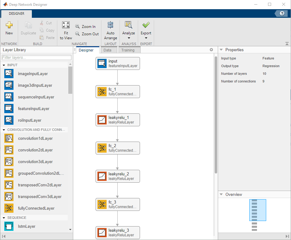
Different network architectures can help with the task of pricing barrier options using a Heston model. Choosing a neural network architecture requires balancing computation time against accuracy. This example uses multiple, fully-connected layers and Leaky ReLU activations.

numFeatures = size(inputs,2);
layers = [
    featureInputLayer(numFeatures,Normalization='zscore')    
    fullyConnectedLayer(32,WeightsInitializer='he')
    leakyReluLayer
    fullyConnectedLayer(32,WeightsInitializer='he')
    leakyReluLayer
    fullyConnectedLayer(32,WeightsInitializer='he')
    leakyReluLayer
    fullyConnectedLayer(1,WeightsInitializer='he')
    leakyReluLayer
    ];

Visualize Network

You can visualize the network using the Deep Network Designer (Deep Learning Toolbox) app or the analyzeNetwork (Deep Learning Toolbox) function.

deepNetworkDesigner(layers)

Train Network

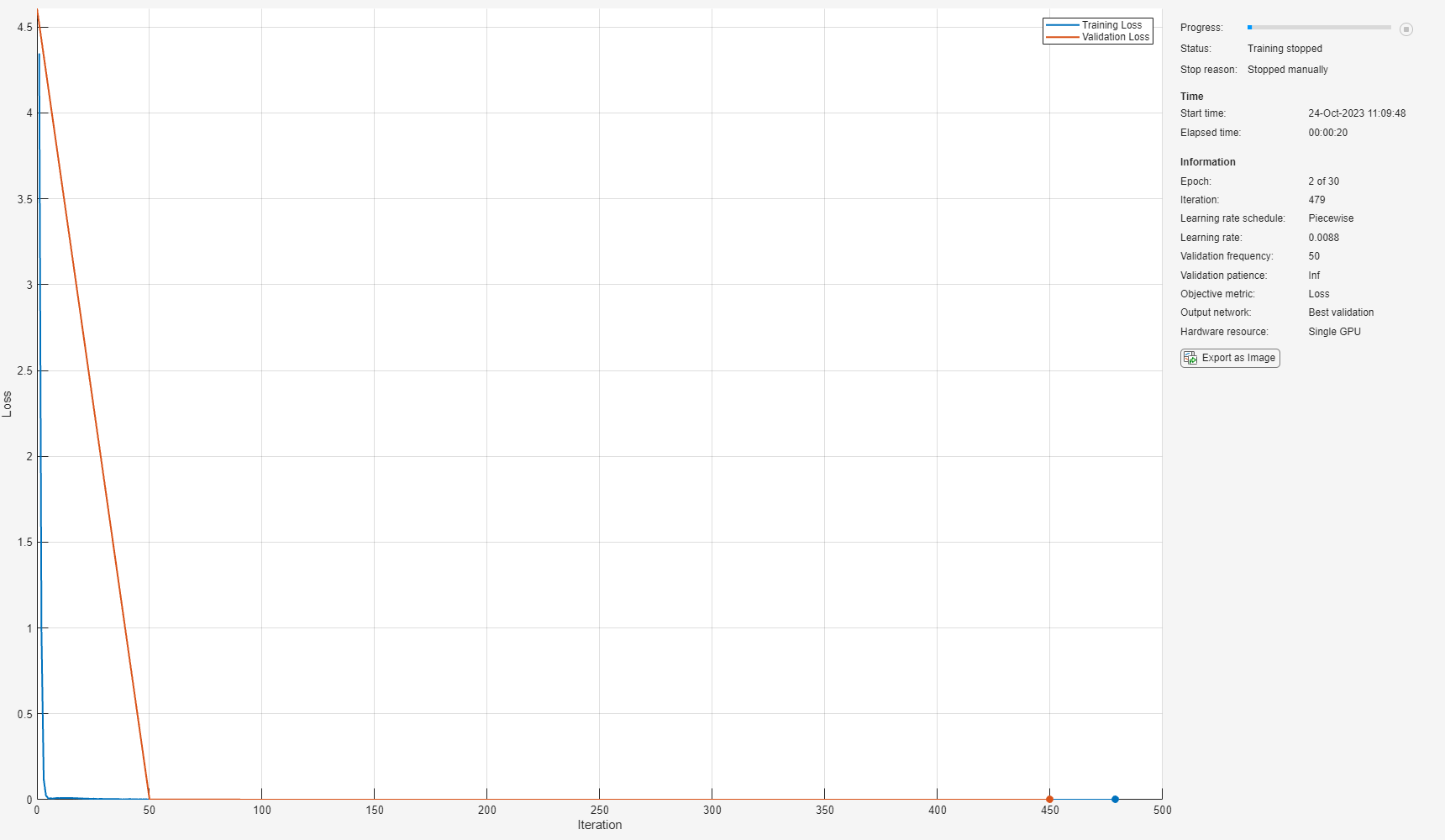
Train the neural network by using the trainnet (Deep Learning Toolbox) function. The function creates a hold-out set to test the trained network and allocates a validation set to monitor the overfitting during the training. By default, trainnet (Deep Learning Toolbox) uses a GPU if one is available; otherwise, it uses a CPU. Training on a GPU requires Parallel Computing Toolbox™ and a supported GPU device. For information, see Deep Learning with MATLAB on Multiple GPUs (Deep Learning Toolbox).

n = size(Price,1);
c = cvpartition(n,Holdout=1/5);     % Hold out 1/5 of the data set for testing
XTrain = inputs(training(c),:);     % 4/5 of the input for training
YTrain = Price(training(c),:);      % 4/5 of the target for training
XTest = inputs(test(c),:);          % 1/5 of the input for testing
YTest = Price(test(c),:);           % 1/5 of the target for testing

nTrain = size(XTrain,1);
idx = randperm(nTrain,floor(nTrain*0.1)); % 10% validation data
XValidation = XTrain(idx,:);
XTrain(idx,:) = [];
YValidation = YTrain(idx,:);
YTrain(idx,:) = [];

opts = trainingOptions('adam', ...
    MaxEpochs=30, ...
    Shuffle='every-epoch', ...
    Plots='none', ...
    Verbose=false, ...
    VerboseFrequency=50, ...
    MiniBatchSize=265, ...
    ValidationData={XValidation,YValidation}, ...
    ValidationFrequency=50, ...
    ValidationPatience=Inf, ...
    L2Regularization=1.9e-7, ...
    InitialLearnRate=8.8e-3, ...
    LearnRateSchedule='piecewise', ...
    LearnRateDropPeriod=4, ...
    LearnRateDropFactor=0.128, ...
    SquaredGradientDecayFactor=0.55, ...
    GradientDecayFactor=0.62);
%opts.ExecutionEnvironment = "gpu";  % When using GPU

doTraining = false;
if doTraining
    % Train the network.
    net = trainnet(XTrain,YTrain,layers,"mean-squared-error",opts);
else
    % Load the pretrained network for the example.
    load('DeepLearningBarrierHeston.mat','net')
end

To avoid waiting for the training, load the pretrained network by setting the doTraining flag to false. To train the networks using trainnet (Deep Learning Toolbox), set the doTraining flag to true. The Training Progress window displays progress when Plots in trainingOptions is set as training-progress.

Test Network

After training the network model, you can use the predict (Deep Learning Toolbox) function to evaluate the test data set containing 30,000 barrier options on this trained network. Compared to the histogram in Calculate Barrier Option Prices Using MonteCarlo Simulation where Monte Carlo simulation takes 0.46 seconds to price each barrier option (3.9 hours to price 30,000 barrier options), after the network model is trained, a data set containing 30,000 barrier option is evaluated in seconds.

% If testing on a GPU, then convert data to a gpuArray.
if opts.ExecutionEnvironment == "gpu" && canUseGPU
    XTest = gpuArray(XTest);
end

YPred = predict(net,XTest);

To assess the performance of the network, calculate the mean-squared error (MSE) value.

mseTest = mean((YTest - YPred).^2)

mseTest = single

2.9402e-06

The following histogram shows the error distribution for the predicted barrier option price using Deep Learning Toolbox™ with respect to the calculated barrier option price using Financial Instrument Toolbox™.

figure
histogram(YTest - YPred, Binwidth=1e-4)
xlabel('Error Distribution')
ylabel('Counts')

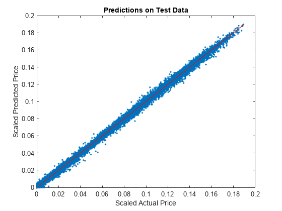
A plot of the calculated prices and predicted prices shows the performance of the network for the Heston model using the test data.

figure
plot(YTest,YPred,'.',[min(YTest),max(YTest)],[min(YTest),max(YTest)],'r')
xlabel('Scaled Actual Price')
ylabel('Scaled Predicted Price')
title('Predictions on Test Data')

References

[1] Goodfellow, I., Y. Bengio, and A. Courville. Deep Learning. MIT Press, 2016.

[2] Niederreiter, H. "Random Number Generation and Quasi-Monte Carlo Methods." Society for Industrial and Applied Mathematics, 1992.