Main Content

ssregest

Estimate state-space model by reduction of regularized ARX model

Description

Estimate State-Space Model

sys = ssregest(tt,nx) estimates a discrete-time state-space model by reduction of a regularized ARX model, using the all the input and output signals in the timetable tt. You can use this syntax for SISO and MIMO systems. The function assumes that the last variable in the timetable is the single output signal. You can also use this syntax to estimate a time-series model if tt contains a single variable that represents the sole output.

For MIMO systems and for timetables that contain more variables than you plan to use for estimation, you must also use name-value arguments to specify the names of the input and output channels you want. For more information, see tt.

To estimate a continuous-time model, set 'Ts' to 0 using name-value syntax.

example

sys = ssregest(u,y,nx,'Ts',Ts) uses the time-domain input and output signals in the comma-separated matrices u,y and the model sample time Ts. The software assumes that the data sample time is also Ts seconds. You can use this syntax for SISO, MISO, and MIMO systems.

Estimating continuous-time models from matrix-based data is not recommended.

example

sys = ssregest(data,nx) uses the time-domain or frequency-domain data in the data object data. Use this syntax especially when you want to estimate a state-space model using frequency-domain or frequency-response data, or when you want to take advantage of the additional information, such as data sample time or experiment labeling, that data objects provide.

Specify Additional Options

sys = ssregest(___,nx,Name,Value) incorporates additional model options specified by one or more name-value arguments. For example, specify input and output signal variable names that correspond with the variables to use for MIMO timetable data using sys = ssregest(data,nx,'InputName',["u1","u2"],'OutputName',["y1","y3"]). Use the 'Form', 'Feedthrough', and 'DisturbanceModel' name-value arguments to modify the default behavior of the A, B, C, D, and K matrices.

example

sys = ssregest(___,opt) specifies estimation options that configure the estimation objective, ARX orders, and order reduction options. This syntax can include any of the input argument combinations in the previous syntaxes.

example

Return Estimated Initial States

[sys,x0] = ssregest(___) returns the value of initial states computed during estimation. This syntax can include any of the input argument combinations in the previous syntaxes.

example

Examples

collapse all

Load the time-domain estimation data, which is contained in the timetable tt.

load sdata2.mat tt2;

Identify a third-order state-space model.

sys = ssregest(tt2,3);

Load estimation data, which is contained in the input/output matrix pair umat2 and ymat2.

load sdata2.mat umat2 ymat2

Estimate a third-order state-space model with input delay. Specify the sample time Ts as 0.1.

sys = ssregest(umat2,ymat2,3,'InputDelay',2,'Ts',0.1);

Load estimation data.

load iddata2 z2;

Specify the order of the regularized ARX model used by the software during estimation. Also, set the estimation focus to simulation.

opt = ssregestOptions('ARXOrder',[100 100 1],'Focus','simulation');

Identify a third-order state-space model.

sys = ssregest(z2,3,opt);

Load estimation data.

load sdata2 tt2;

Obtain the initial state values when identifying a third-order state-space model.

[sys,x0] = ssregest(tt2,3);
x0
x0 = 3×1

    0.1418
   -0.0303
    0.1452

Load data.

load regularizationExampleData eData;

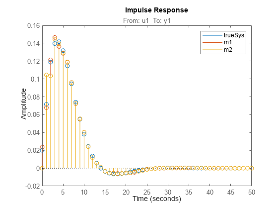
Create a transfer function model used for generating the estimation data (true system).

trueSys = idtf([0.02008 0.04017 0.02008],[1 -1.561 0.6414],1);

Obtain regularized impulse response (FIR) model.

opt = impulseestOptions('RegularizationKernel','DC');
m0 = impulseest(eData,70,opt);

Convert the model into a state-space model and reduce the model order.

m1 = balred(idss(m0),15);

Obtain a second state-space model using regularized reduction of an ARX model.

m2 = ssregest(eData,15);

Compare the impulse responses of the true system and the estimated models.

impulse(trueSys,m1,m2,50);   
legend('trueSys','m1','m2');

MATLAB figure

Input Arguments

collapse all

Estimation data, specified as a uniformly sampled timetable that contains variables representing input and output channels or, for multiexperiment data, a cell array of timetables.

Use Entire Timetable

If you want to use all the variables in tt as input or output channels, and the variables are organized so that the set of input channel variables is followed by the set of output channel variables, then:

  • For SISO systems, specify tt as an Ns-by-2 timetable, where Ns is the number of samples and the two timetable variables represent the measured input channel and output channel respectively.

  • For MIMO systems, specify tt as an Ns-by-(Nu+Ny) timetable, where Nu is the number of inputs and Ny is the number of outputs. The first Nu variables must contain the input channels and the remaining Ny variables must contain the output channels.

    When you are estimating state space or transfer function models, you must also explicitly specify the input and output channels, as the following section describes.

  • For multiexperiment data, specify data as an Ne-by-1 cell array of timetables, where Ne is the number of experiments. The sample times of all the experiments must match.

Use Selected Variables from Timetable

If you want to explicitly identify the input and output channels, such as when you want to use only a subset of the available channels, when the input and output channel variables are intermixed, or when you are estimating a MIMO state-space or transfer function model, use the 'InputName' and 'OutputName' name-value arguments to specify which variables to use as inputs and outputs.

For example, suppose that tt contains six channel variables: "u1", "u2", "u3", and "y1", "y2", "y3". For estimation, you want to use the variables "u1" and "u2" as the inputs and the variables "y1" and "y3" as the outputs. Use the following command to perform the estimation:

sys = ssregest(tt,__,'InputName',["u1" "u2"],'OutputName',["y1" "y3"])

Use Timetable to Estimate Time Series Models

If you want to estimate a time series model rather than an input/output model, use only output variables from tt. You can either specify tt to contain only the output variables that you want, or extract the output variables from tt if tt also contains input variables. The specification approach is similar to that for input/output model estimation.

  • For a single-output system, specify tt as an Ns-by-1 timetable.

  • For a multivariate system, specify tt as an Ns-by-(Ny) timetable. Even if you plan to use all the variables in tt, you must specify all of them using the 'OutputName' name-value argument so that the software does not interpret them as input variables.

For a timetable tt that has variables beyond what you want to use, such as input variables or additional output variables, specify both the output variables you want to use and, in 'InputName', an empty array.

For example, suppose that tt contains six variables: "u1", "u2", "u3", and "y1", "y2", "y3". For time series estimation, you want to use the output variables "y1" and "y3". Use the following command to perform the estimation:

sys = ssregest(tt,__,'OutputName',["y1" "y3"],'InputName',[])

For more information about working with estimation data types, see Data Domains and Data Types in System Identification Toolbox.

Estimation data, specified for SISO systems as a comma-separated pair of Ns-by-1 real-valued matrices that contain uniformly sampled input and output time-domain signal values. Here, Ns is the number of samples.

For MIMO systems, specify u,y as an input/output matrix pair with the following dimensions:

  • uNs-by-Nu, where Nu is the number of inputs.

  • yNs-by-Ny, where Ny is the number of outputs.

For multiexperiment data, specify u,y as a pair of 1-by-Ne cell arrays, where Ne is the number of experiments. The sample times of all the experiments must match.

For time series data, which contains only outputs and no inputs, specify [],y.

Limitations

  • Matrix-based data does not support estimation from frequency-domain data. You must use a data object such as an iddata object or idfrd object (see data).

  • Using matrices for estimation data is not recommended for continuous-time estimation because the data does not provide the sample time. The software assumes that the data is sampled at 1 Hz. For continuous-time estimation, it is recommended that you convert each matrix to a timetable. For example, to convert the matrices um and ym to a timetable tt with a sample time of 0.5 minutes, use the following command.

    tt = timetable(um,ym,'rowtimes',minutes(0.5*(1:size(u,1))))
    For a more detailed example of converting matrix-based SISO data to a timetable, see Convert SISO Matrix Data to Timetable. For an example of converting a MIMO matrix pair to a timetable, see Convert MIMO Matrix Data to Timetable for Continuous-Time Model Estimation.

    For more information about working with estimation data types, see Data Domains and Data Types in System Identification Toolbox.

Estimation data object, specified as an iddata object, an frd object, or an idfrd object that contains uniformly sampled input and output values. For time series models, data can contain only output values. By default, the software sets the sample time of the model to the sample time of the estimation data.

For multiexperiment data, the sample times and intersample behavior of all the experiments must match.

For time-domain estimation, data must be an iddata object containing the input and output signal values.

For frequency-domain estimation, data can be one of the following:

  • Recorded frequency response data (frd (Control System Toolbox) or idfrd)

  • iddata object with properties specified as follows:

    • InputData — Fourier transform of the input signal

    • OutputData — Fourier transform of the output signal

    • Domain'Frequency'

    • Ts — Nonzero

Order of the estimated model, specified as a positive scalar or vector.

If nx is a vector, then ssregest creates a plot which you can use to choose a suitable model order. The plot shows the Hankel singular values for models of chosen values in the vector. States with relatively small Hankel singular values can be safely discarded. A default choice is suggested in the plot.

You can also specify nx = 'best', as in ssregest(data,'best'), in which case the optimal order is chosen automatically in the 1:10 range.

Estimation options for ssregest, specified as an options set you create using ssregestOptions.

Name-Value Arguments

Specify optional pairs of arguments as Name1=Value1,...,NameN=ValueN, where Name is the argument name and Value is the corresponding value. Name-value arguments must appear after other arguments, but the order of the pairs does not matter.

Before R2021a, use commas to separate each name and value, and enclose Name in quotes.

Example: sys = ssregest(z2,3,'InputDelay',2) specifies a delay of 2 sampling periods.

Sample time of the model, specified as 0 or equal to the sample time of data.

For continuous-time models, use Ts = 0. For discrete-time models, specify Ts as a positive scalar whose value is equal to the data sample time.

Input delay for each input channel, specified as a numeric vector. For continuous-time systems, specify input delays in the time unit stored in the TimeUnit property. For discrete-time systems, specify input delays in integer multiples of the sample time Ts. For example, InputDelay = 3 means a delay of three sampling periods.

For a system with Nu inputs, set InputDelay to an Nu-by-1 vector. Each entry of this vector is a numerical value that represents the input delay for the corresponding input channel.

You can also set InputDelay to a scalar value to apply the same delay to all channels.

Type of canonical form of sys, specified as one of the following values:

  • 'modal' — Obtain sys in modal form.

  • 'companion' — Obtain sys in companion form.

  • 'free' — All entries of the A, B and C matrices are treated as free.

  • 'canonical' — Obtain sys in the observability canonical form [1].

Use the Form, Feedthrough and DisturbanceModel name-value pair arguments to modify the default behavior of the A, B, C, D, and K matrices.

Direct feedthrough from input to output, specified as a logical vector of length Nu, where Nu is the number of inputs. If Feedthrough is specified as a logical scalar, it is applied to all the inputs.

Use the Form, Feedthrough and DisturbanceModel name-value pair arguments to modify the default behavior of the A, B, C, D, and K matrices.

Specify whether to estimate the K matrix which specifies the noise component, specified as one of the following values:

  • 'none' — Noise component is not estimated. The value of the K matrix is fixed to zero value.

  • 'estimate' — The K matrix is treated as a free parameter.

DisturbanceModel must be 'none' when using frequency-domain data.

Use the Form, Feedthrough and DisturbanceModel name-value pair arguments to modify the default behavior of the A, B, C, D, and K matrices.

Output Arguments

collapse all

Estimated state-space model of order nx, returned as an idss model object. The model represents:

x˙(t)=Ax(t)+Bu(t)+Ke(t)y(t)=Cx(t)+Du(t)+e(t)

A, B, C, D, and K are state-space matrices. u(t) is the input, y(t) is the output, e(t) is the disturbance and x(t) is the vector of nx states.

All the entries of A, B, C, and K are free estimable parameters by default. D is fixed to zero by default, meaning that there is no feedthrough, except for static systems (nx=0).

Information about the estimation results and options used is stored in the Report property of the model. Report has the following fields:

Report FieldDescription
Status

Summary of the model status, which indicates whether the model was created by construction or obtained by estimation

Method

Estimation command used

InitialState

Handling of initial states during estimation, returned as one of the following values:

  • 'zero' — The initial state was set to zero.

  • 'estimate' — The initial state was treated as an independent estimation parameter.

This field is especially useful when the InitialState option in the estimation option set is 'auto'.

ARXOrder

ARX model orders, returned as a matrix of nonnegative integers [na nb nk].

Fit

Quantitative assessment of the estimation, returned as a structure. See Loss Function and Model Quality Metrics for more information on these quality metrics. The structure has these fields.

  • FitPercent — Normalized root mean squared error (NRMSE) measure of how well the response of the model fits the estimation data, expressed as the percentage fitpercent = 100(1-NRMSE)

  • LossFcn — Value of the loss function when the estimation completes

  • MSE — Mean squared error (MSE) measure of how well the response of the model fits the estimation data

  • FPE — Final prediction error for the model

  • AIC — Raw Akaike Information Criteria (AIC) measure of model quality

  • AICc — Small-sample-size corrected AIC

  • nAIC — Normalized AIC

  • BIC — Bayesian Information Criteria (BIC)

Parameters

Estimated values of model parameters

OptionsUsed

Option set used for estimation. If no custom options were configured, this is a set of default options. See ssregestOptions for more information.

RandState

State of the random number stream at the start of estimation. Empty, [], if randomization was not used during estimation. For more information, see rng.

DataUsed

Attributes of the data used for estimation, returned as a structure with the following fields.

  • Name — Name of the data set

  • Type — Data type

  • Length — Number of data samples

  • Ts — Sample time

  • InterSample — Input intersample behavior, returned as one of the following values:

    • 'zoh' — A zero-order hold maintains a piecewise-constant input signal between samples.

    • 'foh' — A first-order hold maintains a piecewise-linear input signal between samples.

    • 'bl' — Band-limited behavior specifies that the continuous-time input signal has zero power above the Nyquist frequency.

  • InputOffset — Offset removed from time-domain input data during estimation. For nonlinear models, it is [].

  • OutputOffset — Offset removed from time-domain output data during estimation. For nonlinear models, it is [].

For more information on using Report, see Estimation Report.

Initial states computed during estimation, returned as a scalar. If data contains multiple experiments, then x0 is a matrix with each column corresponding to an experiment.

This value is also stored in the Parameters field of the model’s Report property.

More About

collapse all

Modal Form

In modal form, A is a block-diagonal matrix. The block size is typically 1-by-1 for real eigenvalues and 2-by-2 for complex eigenvalues. However, if there are repeated eigenvalues or clusters of nearby eigenvalues, the block size can be larger.

For example, for a system with eigenvalues (λ1,σ±jω,λ2), the modal A matrix is of the form

Am=[λ10000σω00ωσ0000λ2].

Companion Form

In the companion realization, the characteristic polynomial of the system appears explicitly in the rightmost column of the A matrix.

For a system with characteristic polynomial

P(s)=sn+αn1sn1+αn2sn2++α1s+α0,

the corresponding companion A matrix is

Accom=[01000001000001000001α0α1α2α3  αn1],Bccom=[100].

The companion transformation requires that the system be controllable from the first input. The companion form is poorly conditioned for most state-space computations; avoid using it when possible.

Tips

  • ssregest function provides improved accuracy than n4sid for short, noisy data sets.

  • For some problems, the quality of fit using n4sid is sensitive to options, such as N4Horizon, whose values can be difficult to determine. In comparison, the quality of fit with ssregest is less sensitive to its options, which makes ssregest simpler to use.

Algorithms

ssregest estimates a regularized ARX model and converts the ARX model to a state-space model. The software then uses balanced model reduction techniques to reduce the state-space model to the specified order.

References

[1] Ljung, L. System Identification: Theory For the User, Second Edition, Appendix 4A, pp 132-134, Upper Saddle River, N.J: Prentice Hall, 1999.
Version History

Introduced in R2014a

expand all