利用灵活的非线性函数增强已知线性模型

此示例使用:

此示例演示了一种使用神经状态空间模型来改进现有状态空间模型的归一化均方根误差 (NRMSE) 拟合分数的方法。

离散时间状态空间模型的结构为：

$x_{k + 1} = A x_{k} + B u_{k}$

$y_{k} = x_{k}$

这里， $A x_{k} + B u_{k}$ 表示已知的动力学线性部分。您可以根据先前的知识（例如，从物理建模）或先前的线性估计来计算 $A$ 和 $B$ 矩阵。在此示例中，您可以通过添加由神经网络表示的非线性函数 $f (x_{k}, u_{k})$ 来扩展状态转换动态。为此，您可以使用采用自定义神经网络的神经状态空间模型。

离散时间神经状态空间模型的结构为：

$x_{k + 1} = A x_{k} + B u_{k} + f (x_{k}, u_{k})$

$y_{k} = x_{k}$

模型描述

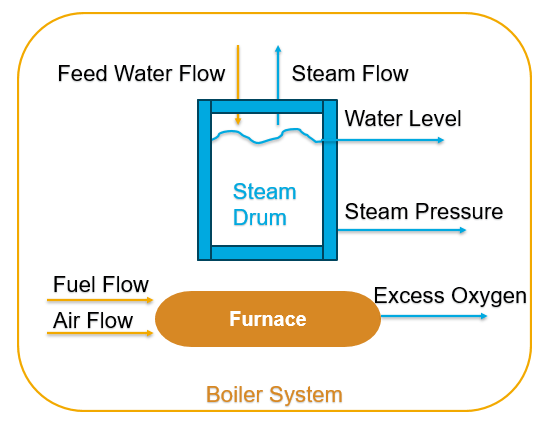
本例考虑了位于伊利诺伊州香槟市的 Abbott 发电厂的蒸汽发生器的动态特性。虽然线性模型提供了良好的基线模型，但它不足以捕获对动态的较小的非线性贡献。因此，您使用的模型是一个具有四个输入和四个输出的非线性系统。它忠实地展示了实际锅炉动力学的所有基本特征，包括非线性、非最小相行为、不稳定性、噪声频谱、时间延迟和负载扰动。有关该模型的详细信息，请参阅 [1]。

数据准备

加载数据集。准备估计和验证数据。

load boiler.mat z
z.OutputName = {'Drum Pressure', 'Excess Oxygen Level', ...
   'Drum Water Level','Steam Flow Rate'};
z.InputName = {'Fuel Flow Rate', 'Air Flow Rate', ...
   'Feed Water Flow Rate','Load Disturbance'};
ze = z(1:7000);
ze.Name = "estimation data";
zv = z(7001:end); 
zv.Name = "validation data";

显示数据集。

idplot(ze,zv)
legend show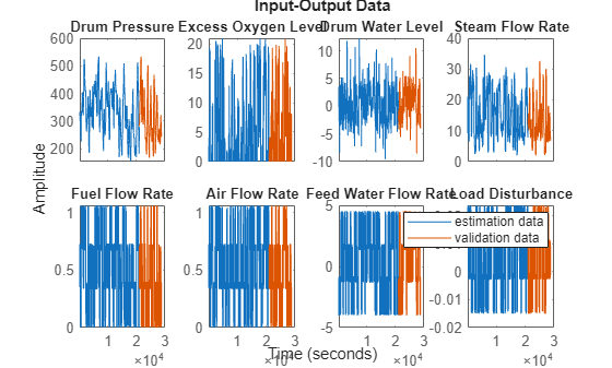

为了确保所有特征具有相同的比例，请对数据集进行规范化。这有助于避免训练期间的数值错误。

ze.y = normalize(ze.y);
ze.u = normalize(ze.u);
zv.y = normalize(zv.y);
zv.u = normalize(zv.u);

线性模型估计

要估计线性模型，您可以使用：

包含简化假设的经验或物理定律
Simulink® 中的数字系统，并使其在标称工作条件下线性化
ssest 函数

在此示例中，您使用 ssestOptions 设置训练选项，并使用 ssest 函数训练四阶线性状态空间模型。

nx = 4;
opt = ssestOptions;
opt.Focus = "simulation";
opt.OutputWeight = eye(nx);
opt.EstimateCovariance = false;
opt.SearchMethod = "lm";

rng(1)
sysd = ssest(ze,nx,opt,DisturbanceModel="none",Ts=3);

转换模型，使其具有 y=x 作为输出方程。这对于稍后创建神经状态空间模型是必需的。

linsys = ss2ss(sysd,sysd.C)

linsys =
  Discrete-time identified state-space model:
    x(t+Ts) = A x(t) + B u(t) + K e(t)
       y(t) = C x(t) + D u(t) + e(t)
 
  A = 
              x1         x2         x3         x4
   x1     0.9963    0.02005  -0.003057   -0.05075
   x2    0.02933     0.7955  -0.005347    0.02414
   x3    0.03075    -0.0462     0.9575    -0.1081
   x4    0.05099   -0.02074   0.007758     0.8997
 
  B = 
       Fuel Flow Ra  Air Flow Rat  Feed Water F  Load Disturb
   x1       0.06703     -0.009903      0.004164       0.01035
   x2       -0.1894        0.1014      -0.02146      0.008553
   x3       0.03703       0.02013       0.03299       0.06205
   x4       0.04863       0.01055      -0.01498       0.06012
 
  C = 
                 x1  x2  x3  x4
   Drum Pressur   1   0   0   0
   Excess Oxyge   0   1   0   0
   Drum Water L   0   0   1   0
   Steam Flow R   0   0   0   1
 
  D = 
                 Fuel Flow Ra  Air Flow Rat  Feed Water F  Load Disturb
   Drum Pressur             0             0             0             0
   Excess Oxyge             0             0             0             0
   Drum Water L             0             0             0             0
   Steam Flow R             0             0             0             0
 
  K = 
       Drum Pressur  Excess Oxyge  Drum Water L  Steam Flow R
   x1             0             0             0             0
   x2             0             0             0             0
   x3             0             0             0             0
   x4             0             0             0             0
 
Sample time: 3 seconds

Parameterization:
   FREE form (all coefficients in A, B, C free).
   Feedthrough: yes
   Disturbance component: estimate
   Number of free coefficients: 80
   Use "idssdata", "getpvec", "getcov" for parameters and their uncertainties.

Status:                         
Model modified after estimation.
 
Model Properties

将仿真模型响应与验证数据进行比较。

compare(zv,linsys)

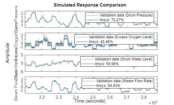
您可以看到线性模型不足以进行估计，因为第二和第三个输出的拟合百分比很差。

非线性模型估计

首先，根据状态方程 $x_{k + 1} = A x_{k} + B u_{k} + f (x_{k}, u_{k})$ 创建用于训练的状态网络。该模型有四个状态、四个输入和一个大小为 10 的隐藏层。

nx = 4;
nu = 4;
nh = 10;

使用示例末尾定义的辅助函数 createSSNN 创建自定义神经网络来表示状态方程。

net = createSSNN(nx,nu,nh);  % x(k+1) = Ax + Bu + f(x,u)

根据线性模型中的值初始化与 A 和 B 对应的权重和偏置。

A = linsys.A;
B = linsys.B;
ind = 7;
net.Learnables{ind,3} = {dlarray(A)};  % weight for A
net.Learnables{ind+1,3} = {dlarray(zeros(nx,1))}; % bias for A
net.Learnables{ind+2,3} = {dlarray(B)}; % weight for B
net.Learnables{ind+3,3} = {dlarray(zeros(nx,1))}; % bias for B
plot(net)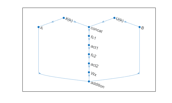

Figure contains an axes object. The axes object contains an object of type graphplot.

使用idNeuralStateSpace创建神经状态空间模型，使用与线性模型相同的采样时间。将创建的自定义网络指定为模型的状态网络。

nss = idNeuralStateSpace(nx,NumInputs=nu,Ts=linsys.Ts);
nss.StateNetwork = net;

Warning: By default, "X(k)" layer is used as state and "U(k)" layer is used as input. If this is not the case, consider using "setNetwork" to assign the layer names.

为了避免警告，您可以使用 setNetwork 函数。

nss = setNetwork(nss,"state",net,xName='X(k)',uName='U(k)');

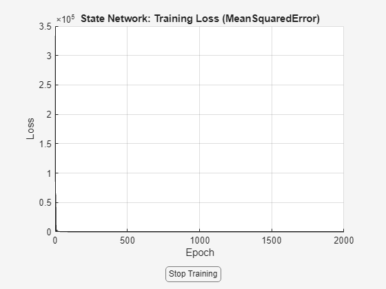
使用nssTrainingOptions设置训练选项，使用nlssest训练模型。

opts = nssTrainingOptions('adam');
opts.MaxEpochs = 2000;
opts.LearnRate = 0.07;
opts.WindowSize = 150;
opts.Overlap = 30;
opts.LossFcn = "MeanSquaredError";
opts.LearnRateSchedule = "piecewise";
opts.LearnRateDropFactor = 0.6;
opts.LearnRateDropPeriod = 600;

sys = nlssest(ze,nss,opts)

Figure Loss contains an axes object and another object of type uigridlayout. The axes object with title State Network: Training Loss (MeanSquaredError), xlabel Epoch, ylabel Loss contains an object of type animatedline.

Generating estimation report...done.

sys =

Discrete-time Neural ODE in 4 variables
     x(t+1) = f(x(t),u(t))
       y(t) = x(t) + e(t)
 
f(.) network:
  Deep network with 4 fully connected, hidden layers
  Activation function: sigmoid
 
Variables: x1, x2, x3, x4
Sample time: 3 seconds
 
Status:                                          
Estimated using NLSSEST on time domain data "ze".
Fit to estimation data: [82.5;75.63;72.04;87.08]%
FPE: 2.476e-06, MSE: 0.1849                      

Model Properties

将仿真的线性和非线性模型响应与验证数据进行比较。

compare(zv,linsys,sys)

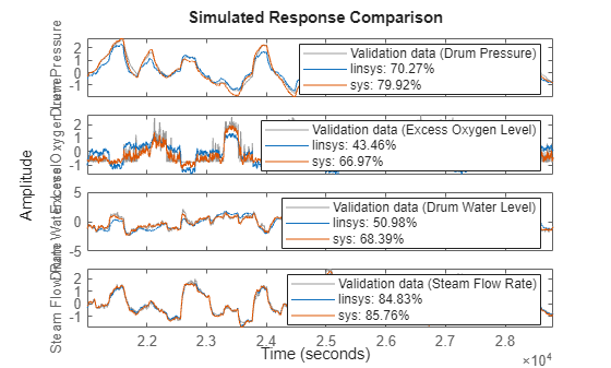
验证 A 和 B 对应的权重是否与线性模型的权重相同。

A_trained = extractdata(sys.StateNetwork.Learnables.Value{7});
isequal(A,A_trained)

ans = logical
   1

B_trained = extractdata(sys.StateNetwork.Learnables.Value{9});
isequal(B,B_trained)

ans = logical
   1

您可以观察到，神经状态空间模型成功捕获了未建模的动态，并且线性部分已固定。

创建神经网络的函数

创建一个代表 $x (k + 1) = A x + B u + f (x, u)$ 的自定义神经网络。

function net = createSSNN(nx,nu,nh)
net = dlnetwork;

% Input layers for x and u
tempLayers = featureInputLayer(nx,"Name","X(k)");
net = addLayers(net,tempLayers);
tempLayers = featureInputLayer(nu,"Name","U(k)");
net = addLayers(net,tempLayers);

% Layers for f(x,u)
tempLayers = [
    concatenationLayer(1,2,"Name","concat") 
    fullyConnectedLayer(nh,"Name","fc1")
    sigmoidLayer("Name","act1")
    fullyConnectedLayer(nh,"Name","fc2")
    sigmoidLayer("Name","act2")
    fullyConnectedLayer(nx,"Name","Wx")];
net = addLayers(net,tempLayers);

% Layers for Ax
tempLayers = fullyConnectedLayer(nx,"Name","A");
tempLayers.WeightLearnRateFactor = 0; % Fix linear component of model
tempLayers.BiasLearnRateFactor = 0;
net = addLayers(net,tempLayers);

% Layers for Bu
tempLayers = fullyConnectedLayer(nx,"Name","B");
tempLayers.WeightLearnRateFactor = 0; % Fix linear component of model
tempLayers.BiasLearnRateFactor = 0;
net = addLayers(net,tempLayers);

% Layers for f(x,u)
tempLayers = additionLayer(3,"Name","addition");
net = addLayers(net,tempLayers);

% Connect all branches of the network to create the network graph
net = connectLayers(net,"X(k)","concat/in1");
net = connectLayers(net,"X(k)","A");
net = connectLayers(net,"U(k)","concat/in2");
net = connectLayers(net,"U(k)","B");
net = connectLayers(net,"A","addition/in1");
net = connectLayers(net,"B","addition/in2");
net = connectLayers(net,"Wx","addition/in3");

% Initialize the network
net = initialize(net);
end

参考资料

1] G. Pellegrinetti and J. Benstman, Nonlinear Control Oriented Boiler Modeling - A Benchmark Problem for Controller Design, IEEE Tran.Control Systems Tech.Vol.4No.1 Jan.1996

另请参阅

对象

idNeuralStateSpace

函数

nssTrainingOptions | nlssest | idplot | ss2ss | ssest | compare | ssestOptions | setNetwork