Model Shack-Hartmann Wavefront Sensor

Shack-Hartmann Wavefront Sensor Principles

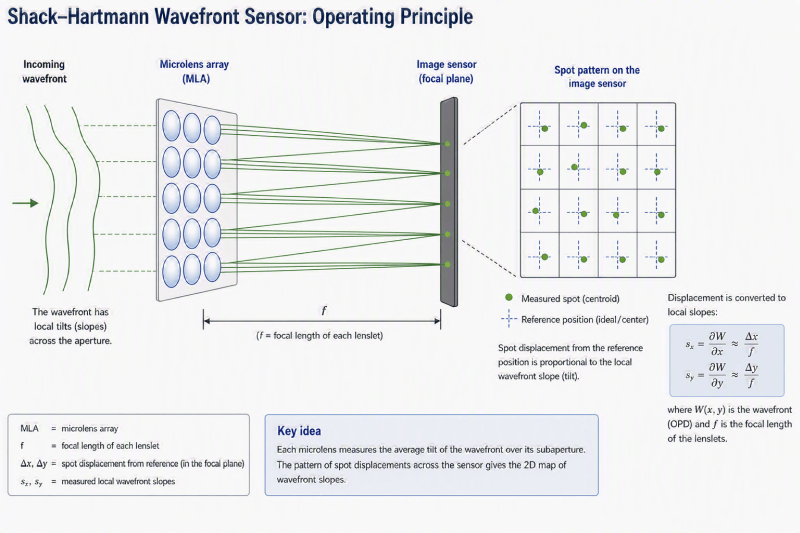
A Shack-Hartmann Wavefront Sensor (WFS) [1] consists of a microlens array (MLA) and an image sensor placed at the MLA focal plane. Each lenslet samples a small portion of the incoming wavefront and focuses it to a spot on the sensor. For a perfect plane wave, all spots land at regular grid positions. When the wavefront is aberrated, each spot shifts by an amount proportional to the local wavefront slope [2]. By measuring the displacement of every spot relative to a reference position, the WFS recovers the two-dimensional slope field ($$\partial W/\partial x$$, $$\partial W/\partial y$$) and reconstructs the wavefront $$W(x,y)$$ [5].

Create Wavefront Sensor

Create a Shack-Hartmann WFS by pairing the Thorlabs MLA150-5C [3] microlens array with the WFS31-5C [4] image sensor.

Define Microlens Array Surface

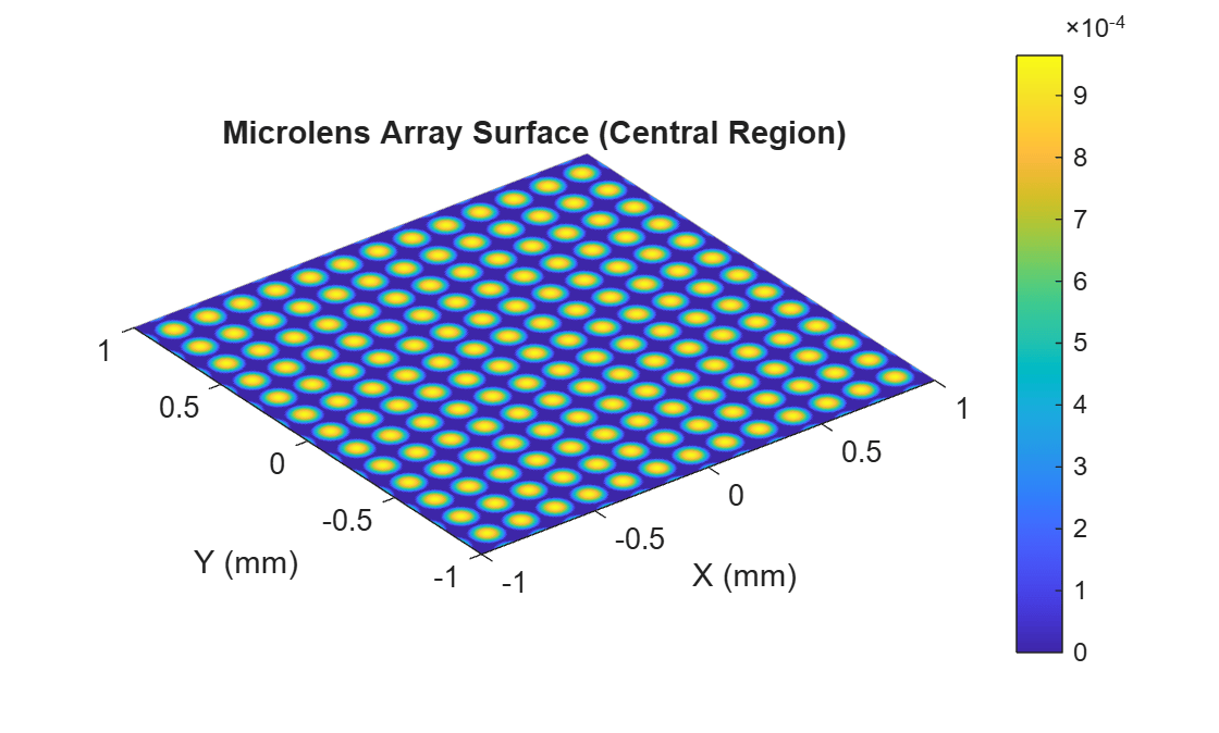
Model the MLA as a grid surface that defines the sag profile of the lenslet array. Define the microlens parameters from the Thorlabs MLA150-5C specification:

Specify the MLA150-5C microlens array parameters.

lensletPitch = 0.150;
lensletActiveSize = 0.140;
radiusOfCurvature = 2.54;

Generate the sag surface over a 2-millimeter region by using the microlensArraySurface helper function, included in the supporting project file attached to this example.

plotSize = 2;
nPoints = round(plotSize / lensletPitch) * 20;
[Zsag,X,Y] = microlensArraySurface(plotSize,nPoints,lensletPitch,lensletActiveSize,radiusOfCurvature);

Visualize the central region of the MLA sag profile to show the lenslet pattern.

figure;
surf(X,Y,Zsag,EdgeColor="none");
xlabel("X (mm)");
ylabel("Y (mm)");
zlabel("Sag (mm)");
title("Microlens Array Surface (Central Region)");
colormap("parula");
colorbar;
axis equal;

Build Wavefront Sensor

Create the wavefront sensor and extract its parameters by using the createSHWavefrontSensor helper function, attached to this example as a supporting file. The helper function builds the complete WFS optical system by using the Thorlabs specifications: 150 micrometer pitch, 5.6 millimeter focal length, and a 73-by-45 grid of active lenslets.

opsysWFS = createSHWavefrontSensor;
wfsParams = opsysWFS.UserData;
designWavelength = opsysWFS.Wavelengths;
pitch = wfsParams.MicroLensArray.LensletPitch;
nLensX = wfsParams.NumLenslets(1);
nLensY = wfsParams.NumLenslets(2);

Measure Wavefront

To measure the optical path difference (OPD) over the exit pupil of an optical system by using a Shack-Hartmann sensor, you must place the microlens array in a plane conjugate to the exit pupil.

For most optical systems, the exit pupil is virtual and located within the system. A relay lens is therefore used to form an image of the exit pupil at a convenient physical location. This relay can also scale the pupil to match the size of the wavefront sensor.

In this configuration, the wavefront sensor measures the combined OPD of the system under test and the relay:

You can measure the relay OPD separately and subtract it to isolate the system under test, but this requires the relay OPD to remain constant across input ray angles. Simpler relay designs can vary significantly with field angle, so an on-axis relay measurement may not represent its behavior under general illumination.

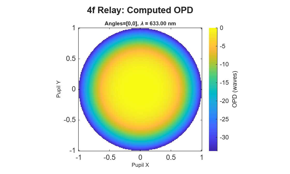
For this reason, this example does not subtract the relay OPD from the combined measurement. Instead, you compare the measured relay OPD directly with the theoretical OPD computed by using the opd function to validate consistency.

Create 4f Relay Lens

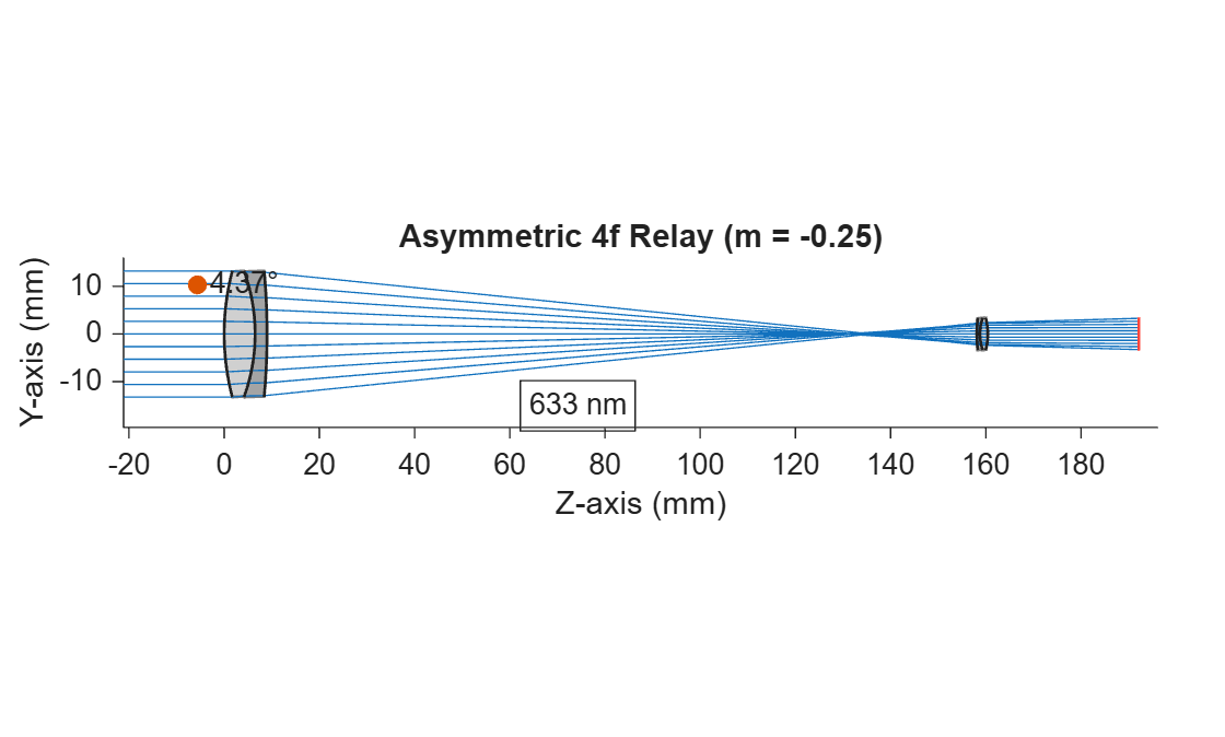
Use an asymmetric 4f relay with magnification $$m=-0.25$$. The relay uses two achromatic doublets: D1 ($$f_1=125$$ millimeters) collimates the beam and D2 ($$f_2=32$$ millimeters) re-images it onto the MLA. The create4fRelayLens helper function builds this relay system. This function is attached to this example as a supporting file.

Create the relay system and add the image sensor by using the addImageSensor function.

opsysRelay = create4fRelayLens;
addImageSensor(opsysRelay,Resolution=wfsParams.ImageSensor.SensorResolution,RectangleSize=wfsParams.ImageSensor.SensorSize);

Visualize the relay by using the view2d function and display traced rays by using the addRays function.

hvRelay = view2d(opsysRelay);
addRays(hvRelay);

Compute the wavefront error of this relay by using the opd function.

opdRelayOnly = opd(opsysRelay);
show(opdRelayOnly,Style="map",Parent=figure);
title("4f Relay: Computed OPD");

Measure Wavefront Slope

To demonstrate how the WFS measures wavefront slopes, attach it to the 4f relay lens. The relay introduces spherical aberration, which displaces each lenslet spot by an amount proportional to the local wavefront slope.

Create a combined relay and WFS opticalSystem object.

opsysRelayWFS = opticalSystem(Name="Relay + WFS",Wavelengths=designWavelength);

Remove the image plane from the relay. Use the distanceAfter function to record the gap and the changeGap function to zero the trailing distance before adding the relay to the combined system.

opsysRelay2 = copy(opsysRelay);
remove(opsysRelay2);
distanceToWFS = distanceAfter(opsysRelay2,numel(opsysRelay2.Components));
changeGap(opsysRelay2,numel(opsysRelay2.Components),0);
add(opsysRelayWFS,opsysRelay2);

Place the microlens array where the image plane of the relay will be. Since the relay is image-space telecentric, the OPD is computed at the image plane. Reduce the distance by the thickness of the WFS substrate.

relayToMLADist = distanceToWFS - opsysWFS.Components(1).Thickness;
changeGap(opsysRelayWFS,1,relayToMLADist);
add(opsysRelayWFS,opsysWFS);

Compute Spot Field

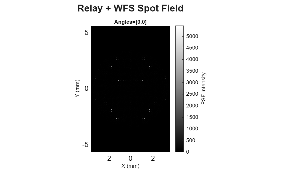
The spot field shows the pattern of focused spots on the image sensor when a collimated beam passes through the relay and WFS. Each lenslet focuses a portion of the demagnified beam to a spot on the sensor. The displacement of each spot from a regular grid reveals the wavefront aberration introduced by the relay.

Compute the geometric PSF of the combined relay and WFS system by using the psf function and display the result.

pixelSizeUM = wfsParams.ImageSensor.PixelSize*1000;
sensorRes = wfsParams.ImageSensor.SensorResolution;
psfRelayWFS = psf(opsysRelayWFS,Method="Geometric",OutputResolution=[sensorRes(2) sensorRes(1)],PixelSize=pixelSizeUM,PupilDensityScale=1e-1);
hpsf = show(psfRelayWFS,Parent=figure);
hpsf.Colormap = colormap("gray");
title("Relay + WFS Spot Field");

Compute Spot Displacements

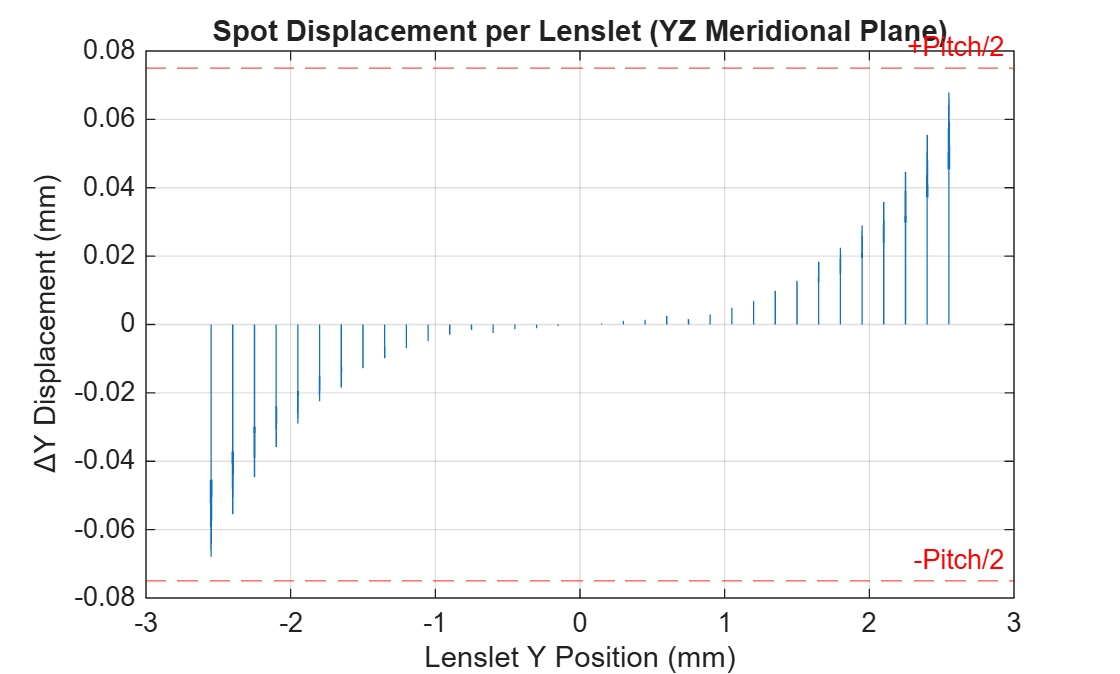
Trace rays in the YZ-meridional plane through the WFS alone as a reference and through the relay combined with the WFS as a test. The displacement of each spot from its reference position is proportional to the local wavefront slope.

Compute and plot the spot displacements by using the computeYAxisDisplacements helper function, included in the supporting project file attached to this example. The quiver plot shows the measured spot displacement at each lenslet. The arrows grow faster near the edges, revealing the spherical aberration of the relay.

computeYAxisDisplacements(opsysWFS,opsysRelayWFS,pitch,[nLensX nLensY]);

Measure Wavefront Error for Relay System

To quantify the relay aberration, measure the wavefront error by comparing spot centroids from the WFS alone as a reference with those from the combined relay and WFS as a test, then reconstruct the wavefront from the centroid displacements.

Compute Reference Centroids

Create a samplingGrid object and trace a collimated on-axis beam through the WFS alone by using the traceRays function. Compute the spot centroids by using the computeLensletCentroids helper function, included in the supporting project file attached to this example. The resulting centroids define the zero-aberration reference positions.

sg = samplingGrid("square",201);
rbRef = traceRays(opsysWFS,SamplingGrid=sg);
[refCentX,refCentY] = computeLensletCentroids(rbRef,pitch,[nLensX nLensY]);

Compute Centroids for System Under Test

Trace the same collimated beam through the combined relay and WFS. The relay aberration displaces the spots relative to the reference positions.

rbTest = traceRays(opsysRelayWFS,SamplingGrid=sg);
[testCentX,testCentY] = computeLensletCentroids(rbTest,pitch,[nLensX nLensY]);

Reconstruct Wavefront Error by Using Southwell's Method

Reconstruct the wavefront by using the Southwell zonal algorithm [5]. The centroid displacement $$\Delta x$$ at each lenslet is proportional to the local wavefront slope: $$\partial W/\partial x=\Delta x/f$$, where $$f$$ is the MLA focal length.

The Southwell method applies the trapezoidal integration rule between adjacent lenslets:

where $$p$$ is the lenslet pitch. These equations form the sparse linear system $$AW=S$$, which is solved in a least-squares sense to recover the wavefront.

Perform the Southwell wavefront reconstruction from centroid displacements by using the southwellReconstruction helper function, included in the supporting project file attached to this example. Convert the result from millimeters to waves.

fMLA = wfsParams.MicroLensArray.FocalLength;
wavelengthMM = opsysWFS.Wavelengths * 1e-6;
opdReconMM = southwellReconstruction(refCentX,refCentY,testCentX,testCentY,pitch,fMLA);
bothValid = ~isnan(opdReconMM);
opdReconWaves = opdReconMM / wavelengthMM;

Compare WFS Measurement with Ground Truth

To ensure consistent evaluation conditions, recompute the OPD by using a square sampling grid that matches the number of active lenslets along the shorter sensor axis. This ensures the opd function samples the pupil at the same spatial density as the WFS, avoiding oversampling at the pupil edge that would inflate the RMS.

Compute the reference OPD and the reconstructed wavefront statistics.

sgCompare = samplingGrid("square",nLensY);
opdCompare = opd(opsysRelay,SamplingGrid=sgCompare);
rmsRecon = std(opdReconWaves(bothValid),0,"all");
pvRecon = max(opdReconWaves(bothValid),[],"all") - min(opdReconWaves(bothValid),[],"all");

Display the computed and reconstructed OPD maps side by side.

tcl = tiledlayout(1,2,Parent=figure);
show(opdCompare,Style="map",NumPointsPerAxis=nLensY,Parent=tcl);
title("Computed");
nexttile(tcl);

Normalize the reconstructed wavefront to pupil coordinates and display the OPD map.

xCoords = ((1:nLensX) - (nLensX + 1)/2) * pitch;
yCoords = ((1:nLensY) - (nLensY + 1)/2) * pitch;
[colIdx,rowIdx] = find(bothValid');
pupilRadius = max(max(abs(xCoords(colIdx))),max(abs(yCoords(rowIdx))));
xNorm = xCoords / pupilRadius;
yNorm = yCoords / pupilRadius;
imagesc(xNorm,yNorm,opdReconWaves,AlphaData=double(bothValid),AlphaDataMapping="none");
ax = gca;
ax.YDir = "normal";
axis(ax,"square");
xlim(ax,[-1 1]);
ylim(ax,[-1 1]);
cb = colorbar(ax);
cb.Box = "off";
cb.Label.String = "OPD (waves)";
title("Reconstructed"," ",FontSize=14);
xlabel("Pupil X");
ylabel("Pupil Y");
sgtitle("4f Relay Wavefront: Computed vs Measured");

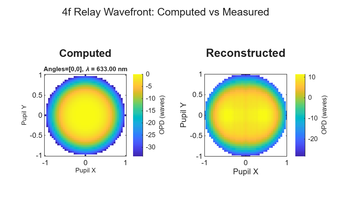
The WFS reconstruction closely matches the computed OPD when both use the same spatial sampling density across the pupil. Any residual discrepancy arises from the finite lenslet aperture, which spatially averages the wavefront slope within each subaperture and limits the ability to resolve high spatial frequency aberrations.

disp("OPD Computed:   RMS = " + round(opdCompare.RMS,4) + " waves, PV = " + round(opdCompare.PeakToValley,4) + " waves")

OPD Computed:   RMS = 10.1077 waves, PV = 33.7234 waves

disp("OPD Measured:   RMS = " + round(rmsRecon,4) + " waves, PV = " + round(pvRecon,4) + " waves")

OPD Measured:   RMS = 9.988 waves, PV = 39.7628 waves

References

[1] RP Photonics. "Shack-Hartmann Wavefront Sensors." RP Photonics Encyclopedia. Accessed June 8, 2026. https://www.rp-photonics.com/shack_hartmann_wavefront_sensors.html.

[2] Platt, Ben C., and Roland Shack. "History and Principles of Shack-Hartmann Wavefront Sensing." Journal of Refractive Surgery 17, no. 5 (2001): S573–S577. https://doi.org/10.3928/1081-597X-20010901-13.

[3] Thorlabs. "MLA150-5C-M Mounted Microlens Array." Thorlabs Product Catalog. Accessed June 8, 2026. https://www.thorlabs.com/thorproduct.cfm?partnumber=MLA150-5C-M.

[4] Thorlabs. "WFS31-5C Shack-Hartmann Wavefront Sensor." Thorlabs Product Catalog. Accessed June 8, 2026. https://www.thorlabs.com/thorproduct.cfm?partnumber=WFS31-5C.

[5] Southwell, William H. "Wave-Front Estimation from Wave-Front Slope Measurements." Journal of the Optical Society of America 70, no. 8 (1980): 998–1006. https://doi.org/10.1364/JOSA.70.000998.