Unsupervised Medical Image Denoising Using CycleGAN

This example uses:

This example shows how to generate high-quality high-dose computed tomography (CT) images from noisy low-dose CT images using a CycleGAN neural network.

X-ray CT is a popular imaging modality used in clinical and industrial applications because it produces high-quality images and offers superior diagnostic capabilities. To protect the safety of patients, clinicians recommend a low radiation dose. However, a low radiation dose results in a lower signal-to-noise ratio (SNR) in the images, and therefore reduces the diagnostic accuracy.

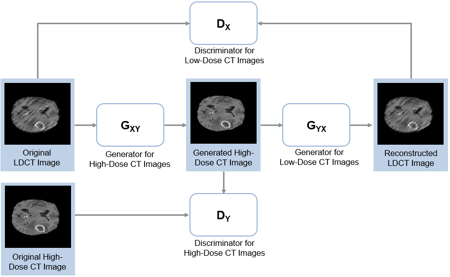
Deep learning techniques can improve the image quality for low-dose CT (LDCT) images. Using a generative adversarial network (GAN) for image-to-image translation, you can convert noisy LDCT images to images of the same quality as regular-dose CT images [1]. For this application, the source domain consists of LDCT images and the target domain consists of regular-dose images. For more information, see Get Started with GANs for Image-to-Image Translation.

CT image denoising requires a GAN that performs unsupervised training because clinicians do not typically acquire matching pairs of low-dose and regular-dose CT images of the same patient in the same session. This example uses a cycle-consistent GAN (CycleGAN) trained on patches of image data from a large sample of data. For a similar approach using a UNIT neural network trained on full images from a limited sample of data, see Unsupervised Medical Image Denoising Using UNIT.

Flowchart showing how the two generators and two discriminators use the real and generated low-dose and high-dose images.

Download AAPM Grand Challenge Data Set

This example uses data from the Low Dose GT Grand Challenge (AAPM) [2, 3, 4]. The data includes pairs of full dose (high-dose) abdominal CT scans and simulated quarter dose (low-dose) abdominal CT scans.

dataDir = fullfile(tempdir,"AAPMGC_LD2HD");
if ~exist(dataDir,"dir")
    mkdir(dataDir);
end

Download the data for this example from the AAPM Grand Challenge Data Repository. Download the files named "QD_3mm_sharp.zip" and "FD_3mm_sharp.zip" and extract the contents of the ZIP files into the folder specified by dataDir.

Create Datastores for Training and Testing

The AAPM Grand Challenge data set provides pairs of low-dose and high-dose CT images. However, the CycleGAN architecture requires unpaired data for unsupervised learning. This example simulates unpaired training and validation data by partitioning images such that the patients used to obtain low-dose CT and high-dose CT images do not overlap. The example retains pairs of low-dose and regular-dose images for testing.

Partition Data

Split the data into training and test data sets using the getLDHDFiles helper function. This function is attached to the example as a supporting file. The helper function splits the data such that there is roughly equal representation of the two types of images. Approximately 80% of the data is used for training and 20% is used for testing. Because of the limited amount of data, the example does not use data for validation.

When you successfully download and extract the data, the training data set has 1,923 pairs of low-dose and high-dose images, and the test set has 455 pairs of low-dose and high-dose images.

[filesTrainHD,filesTrainLD,filesTestLD,filesTestHD] = getLDHDFiles(dataDir);
disp("Number of low-dose training images: "+numel(filesTrainLD));

Number of low-dose training images: 1923

disp("Number of high-dose training images: "+numel(filesTrainHD));

Number of high-dose training images: 1923

disp("Number of low-dose test images: "+numel(filesTestLD));

Number of low-dose test images: 455

disp("Number of high-dose test images: "+numel(filesTestHD));

Number of high-dose test images: 455

Create Image Datastores

Create image datastores that contain training and validation images for both domains, namely low-dose CT images and high-dose CT images. The data set consists of DICOM images, so read the data using the custom ReadFcn name-value argument.

exts = ".IMA";
readFcn = @(x)dicomread(x);
imdsTrainLD = imageDatastore(filesTrainLD,FileExtensions=exts,ReadFcn=readFcn);
imdsTrainHD = imageDatastore(filesTrainHD,FileExtensions=exts,ReadFcn=readFcn);
imdsTestLD = imageDatastore(filesTestLD,FileExtensions=exts,ReadFcn=readFcn);
imdsTestHD = imageDatastore(filesTestHD,FileExtensions=exts,ReadFcn=readFcn);

Preprocess and Augment Data

Define a helper function called preprocessDataHD that preprocesses the high-dose images. The preprocessDataHD helper function resizes the images to 512-by-512 pixels and rescales data to the range [-1, 1].

function hd = preprocessDataHD(hd)
    hd = imresize(hd,[512,512]);
    hd = {rescale(hd,-1,1)};
end

Preprocess the high-dose images using the transform function and the preprocessDataHD helper function.

timdsTrainHD = transform(imdsTrainHD,@preprocessDataHD);
timdsTestHD = transform(imdsTestHD,@preprocessDataHD);

Define a helper function called preprocessDataLD that preprocesses the low-dose images. The preprocessDataLD helper function resizes the images to 512-by-512 pixels and rescales data to the range [-1, 1]. The function also adds Poisson noise to simulate scans with a much lower dose.

function ld = preprocessDataLD(ld)
    ld = imresize(ld,[512,512]);
    for i = 1:10
        ld = imnoise(ld,"poisson");    
    end
    ld = {rescale(ld,-1,1)};
end

Preprocess the low-dose images using the transform function and the preprocessDataLD helper function.

timdsTrainLD = transform(imdsTrainLD,@preprocessDataLD);
timdsTestLD = transform(imdsTestLD,@preprocessDataLD);

Combine the low-dose and high-dose training data by using a randomPatchExtractionDatastore. Shuffle the order of the training data. When reading from this datastore, augment the data using vertical and horizontal reflection.

inputSize = [128 128 1];
patchesPerImage = 32;
augmenter = imageDataAugmenter(RandXReflection=true,RandYReflection=true);

dsTrain = randomPatchExtractionDatastore(shuffle(timdsTrainLD),shuffle(timdsTrainHD), ...
    inputSize(1:2),PatchesPerImage=patchesPerImage,DataAugmentation=augmenter);

Visualize the Data

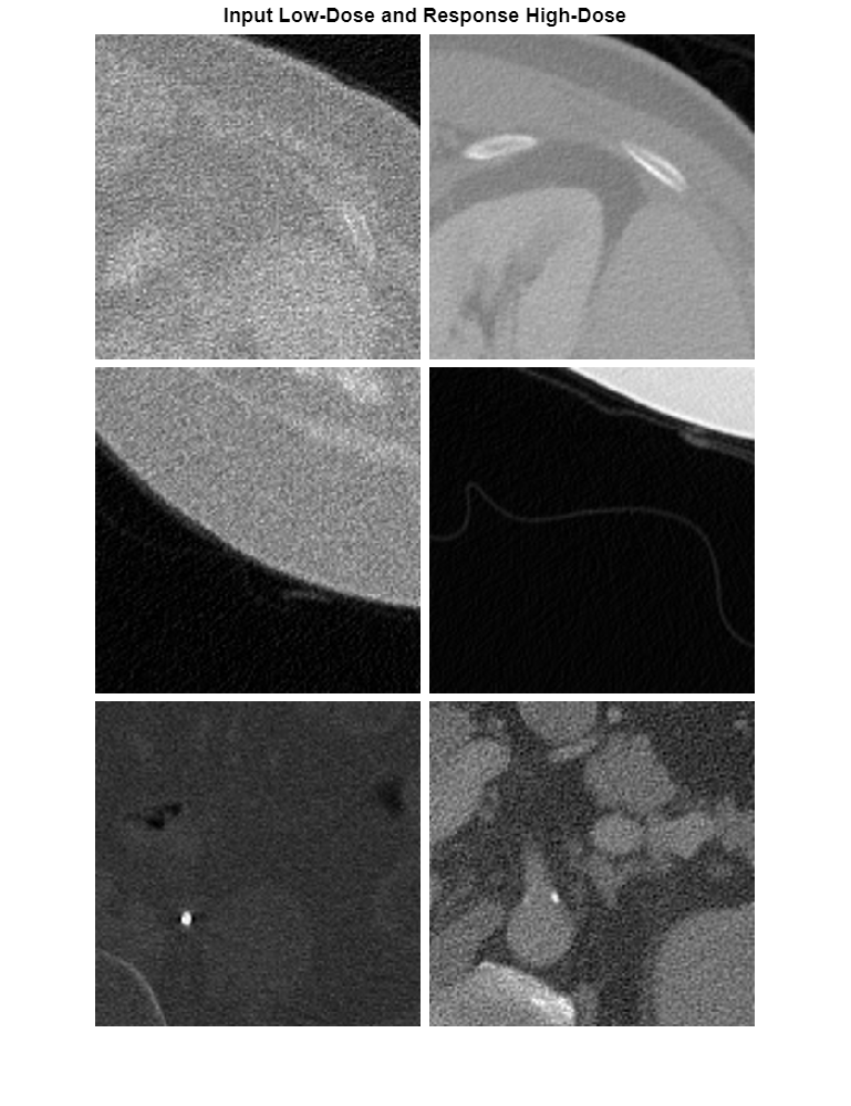
Visualize the low-dose and high-dose image patch pairs from the shuffled training set. Notice that the image pairs of low-dose (left) and high-dose (right) images are unpaired, as they are from different patients.

numImagePairs = 3;
imagePairsTrain = [];
for i = 1:numImagePairs
    imLowAndHighDose = read(dsTrain);
    inputImage = imLowAndHighDose.InputImage{1};
    inputImage = rescale(im2single(inputImage));
    responseImage = imLowAndHighDose.ResponseImage{1};
    responseImage = rescale(im2single(responseImage));
    imagePairsTrain = cat(4,imagePairsTrain,inputImage,responseImage);
end
montage(imagePairsTrain,Size=[numImagePairs 2],BorderSize=4,BackgroundColor="w");
title("Input Low-Dose and Response High-Dose");

Batch Training Data

This example uses a custom training loop. The minibatchqueue (Deep Learning Toolbox) object is useful for managing the mini-batching of observations in custom training loops. The minibatchqueue object also casts data to a dlarray object that enables auto differentiation in deep learning applications.

Define a helper function called concatenateMiniBatch that concatenates a batch of image patches along the batch dimension.

function [out1,out2] = concatenateMiniBatch(im1,im2)
    out1 = cat(4,im1{:});
    out2 = cat(4,im2{:});
end

Create a minibatchqueue object and specify the mini-batch preprocessing function as concatenateMiniBatch. Specify the mini-batch data extraction format as "SSCB" (spatial, spatial, channel, batch). Discard any partial mini-batches with less than miniBatchSize observations.

miniBatchSize = 8;
mbqTrain = minibatchqueue(dsTrain, ...
    MiniBatchSize=miniBatchSize, ...
    MiniBatchFcn=@concatenateMiniBatch, ...
    PartialMiniBatch="discard", ...
    MiniBatchFormat="SSCB");

Create Generator and Discriminator Networks

The CycleGAN consists of two generators and two discriminators. The generators perform image-to-image translation from low-dose to high-dose and vice versa. The discriminators are PatchGAN networks that return the patch-wise probability that the input data is real or generated. One discriminator distinguishes between the real and generated low-dose images and the other discriminator distinguishes between real and generated high-dose images.

Create each generator network using the cycleGANGenerator function. For an input size of 128-by-128 pixels, specify the NumResidualBlocks argument as 6. By default, the function has 3 encoder modules and uses 64 filters in the first convolutional layer.

numResiduals = 6; 
genHD2LD = cycleGANGenerator(inputSize,NumResidualBlocks=numResiduals,NumOutputChannels=1);
genLD2HD = cycleGANGenerator(inputSize,NumResidualBlocks=numResiduals,NumOutputChannels=1);

Create each discriminator network using the patchGANDiscriminator function. Use the default settings for the number of downsampling blocks and number of filters in the first convolutional layer in the discriminators.

discLD = patchGANDiscriminator(inputSize);
discHD = patchGANDiscriminator(inputSize);

Define Loss Functions and Scores

The modelGradients helper function calculates the gradients and losses for the discriminators and generators. This function is defined in the Supporting Functions section of this example.

The objective of the generator is to generate translated images that the discriminators classify as real. The generator loss is a weighted sum of three types of losses: adversarial loss, cycle consistency loss, and fidelity loss. Fidelity loss is based on structural similarity (SSIM) loss. [5]

Specify the weighting factor λ that controls the relative significance of the cycle consistency loss with the adversarial and fidelity losses.

lambda = 10;

The objective of each discriminator is to correctly distinguish between real images (1) and translated images (0) for images in its domain. Each discriminator has a single loss function that relies on the mean squared error (MSE) between the expected and predicted output.

Specify Training Options

Train for 10 epochs.

numEpochs = 10;

Specify the options for Adam optimization. For both generator and discriminator networks, use:

A learning rate of 0.0002
A gradient decay factor of 0.5
A squared gradient decay factor of 0.999

learnRate = 0.0002;
gradientDecay = 0.5;
sqGradientDecayFactor = 0.999;

Initialize Adam parameters for the generators and discriminators.

avgGradGenLD2HD = [];
avgSqGradGenLD2HD = [];
avgGradGenHD2LD = [];
avgSqGradGenHD2LD = [];
avgGradDiscLD = [];
avgSqGradDiscLD = [];
avgGradDiscHD = [];
avgSqGradDiscHD = [];

Display the generated train image patches every 250 iterations and update the training monitor after every 250 iterations.

displayImageFrequency = 250;
updateTrainingMonitorFrequeny = 250;

Calculate the number of iterations to update the training monitor periodically.

numObservationsTrain = numel(filesTrainLD) * patchesPerImage;
numIterationsPerEpoch = floor(numObservationsTrain / miniBatchSize);
numIterations = numEpochs * numIterationsPerEpoch;

Train or Download Model

By default, the example downloads a pretrained version of the CycleGAN generator for low-dose to high-dose CT. The pretrained network enables you to run the entire example without waiting for training to complete.

To train the network, set the doTraining variable in the following code to true. Train the model in a custom training loop. For each iteration:

Read the data for the current mini-batch using the next (Deep Learning Toolbox) function.
Evaluate the model gradients using the dlfeval (Deep Learning Toolbox) function and the modelGradients helper function.
Update the network parameters using the adamupdate (Deep Learning Toolbox) function.
Display the input and translated images for both the source and target domains after each epoch.

Train using a GPU if one is available. Training on a GPU requires a Parallel Computing Toolbox™ license and a supported GPU device. For information on supported devices, see GPU Computing Requirements (Parallel Computing Toolbox). Otherwise, train using the CPU. Training takes about 80 hours on an NVIDIA™ TITAN V GPU with 12 GB of memory.

doTraining = false;

if doTraining
    
    % Set up trainingProgressMonitor to show training metrics and training info 
    monitor = trainingProgressMonitor;
    monitor.Metrics = ["PSNRLowDose","PSNRHighDose","SSIMLowDose","SSIMHighDose"];
    monitor.Info = ["Epoch","Iteration","LearnRate","ExecutionEnvironment"];
    
    groupSubPlot(monitor,"PSNR",["PSNRLowDose","PSNRHighDose"]);
    groupSubPlot(monitor,"SSIM",["SSIMLowDose","SSIMHighDose"]);
    
    monitor.XLabel = "Iteration";
    monitor.Status = "Configuring";
    monitor.Progress = 0;
    
    % Set executionEnvironment and update the trainingProgressMonitor 
    if canUseGPU
        updateInfo(monitor,ExecutionEnvironment="GPU");
    else
        updateInfo(monitor,ExecutionEnvironment="CPU");
    end

    % Create a directory to store checkpoints
    checkpointDir = fullfile("checkpoints/");
    if ~exist(checkpointDir,"dir")
        mkdir(checkpointDir);
    end
    
    % Update the training status on the trainingProgressMonitor
    monitor.Status = "Running";
    
    epoch = 0;
    iteration = 0;
    metricsForMonitoring = {[],[],[],[]};
    psnrTrain = [];
    ssimTrain = [];
    
    while epoch < numEpochs && ~monitor.Stop
        
        epoch = epoch + 1;
        shuffle(mbqTrain);

        % Loop over mini-batches
        while hasdata(mbqTrain) && ~monitor.Stop
            iteration = iteration + 1;

            % Read mini-batch of data
            [imageLD,imageHD] = next(mbqTrain);

            % Convert mini-batch of data to dlarray and specify the dimension labels
            % "SSCB" (spatial, spatial, channel, batch)
            imageLD = dlarray(imageLD,"SSCB");
            imageHD = dlarray(imageHD,"SSCB");

            % If training on a GPU, then convert data to gpuArray
            if canUseGPU
                imageLD = gpuArray(imageLD);
                imageHD = gpuArray(imageHD);
            end

            % Calculate the loss and gradients
            [genHD2LDGrad,genLD2HDGrad,discrXGrad,discYGrad, ...
                genHD2LDState,genLD2HDState,scores,metrics,imagesOutLD2HD,imagesOutHD2LD] = ...
                dlfeval(@modelGradients,genLD2HD,genHD2LD, ...
                discLD,discHD,imageHD,imageLD,lambda);
            genHD2LD.State = genHD2LDState;
            genLD2HD.State = genLD2HDState;

            % Keep track of all batch-wise metrics in current epoch 
            metricsForMonitoring{1} = [metricsForMonitoring{1} metrics{1}];
            metricsForMonitoring{2} = [metricsForMonitoring{2} metrics{2}];
            metricsForMonitoring{3} = [metricsForMonitoring{3} metrics{3}];
            metricsForMonitoring{4} = [metricsForMonitoring{4} metrics{4}];

            % Update parameters of discLD, which distinguishes
            % the generated low-dose CT images from real low-dose CT images
            [discLD.Learnables,avgGradDiscLD,avgSqGradDiscLD] = ...
                adamupdate(discLD.Learnables,discrXGrad,avgGradDiscLD, ...
                avgSqGradDiscLD,iteration,learnRate,gradientDecay,sqGradientDecayFactor);

            % Update parameters of discHD, which distinguishes
            % the generated high-dose CT images from real high-dose CT images
            [discHD.Learnables,avgGradDiscHD,avgSqGradDiscHD] = ...
                adamupdate(discHD.Learnables,discYGrad,avgGradDiscHD, ...
                avgSqGradDiscHD,iteration,learnRate,gradientDecay,sqGradientDecayFactor);

            % Update parameters of genHD2LD, which
            % generates low-dose CT images from high-dose CT images
            [genHD2LD.Learnables,avgGradGenHD2LD,avgSqGradGenHD2LD] = ...
                adamupdate(genHD2LD.Learnables,genHD2LDGrad,avgGradGenHD2LD, ...
                avgSqGradGenHD2LD,iteration,learnRate,gradientDecay,sqGradientDecayFactor);
                        
            % Update parameters of genLD2HD, which
            % generates high-dose CT images from low-dose CT images
            [genLD2HD.Learnables,avgGradGenLD2HD,avgSqGradGenLD2HD] = ...
                adamupdate(genLD2HD.Learnables,genLD2HDGrad,avgGradGenLD2HD, ...
                avgSqGradGenLD2HD,iteration,learnRate,gradientDecay,sqGradientDecayFactor);
            
            %  Every updateTrainingMonitorFrequeny iterations, update 
            %  the training monitor with metrics
            if mod(iteration,updateTrainingMonitorFrequeny) == 0 || iteration == 1
                recordMetrics(monitor,iteration, ...
                    PSNRLowDose = mean(metricsForMonitoring{1}), ...
                    PSNRHighDose = mean(metricsForMonitoring{2}), ...
                    SSIMLowDose = mean(metricsForMonitoring{3}), ...
                    SSIMHighDose = mean(metricsForMonitoring{4}));
                
                metricsForMonitoring = {[],[],[],[]};
            end
            recordMetrics(monitor,iteration);
            updateInfo(monitor, ...
                Epoch = epoch+" of "+numEpochs, ...
                LearnRate = learnRate, ...
                Iteration = iteration+" of "+numIterations);
            monitor.Progress = 100 * iteration/numIterations;

        end

        % Calculate training statistics for whole scans 
        [psnrEpoch,ssimEpoch] = calculateTrainingMetrics_genLD2HD( ...
            timdsTrainLD,timdsTrainHD,genLD2HD);
        
        psnrTrain = [psnrTrain, psnrEpoch];
        ssimTrain = [ssimTrain, ssimEpoch];
        
        % Save the model after each epoch
        [genLD2HD,genHD2LD,discLD,discHD] = gather(genLD2HD,genHD2LD,discLD,discHD);
        save(checkpointDir+filesep+"LD2HDCTCycleGAN-Epoch-"+epoch+".mat", ...
            "genLD2HD","genHD2LD","discLD","discHD");

    end
    
    % Save the final model
    save(checkpointDir+filesep+"LD2HDCTCycleGAN-Epoch-"+epoch+".mat", ...
            "genLD2HD","genHD2LD","discLD","discHD");
    
    % Mark the training as completed on the training monitor
    if monitor.Stop == 1
        monitor.Status = "Training stopped";
    else
        monitor.Status = "Training complete";
    end

else
    net_url = "https://ssd.mathworks.com/supportfiles/" + ...
        "vision/data/LD2HDCTCycleGAN.zip";
    downloadTrainedNetwork(net_url,dataDir);
    load(fullfile(dataDir,"LD2HDCTCycleGAN.mat"));
end

Plot the peak signal-to-noise ratio (PSNR) and multi-scale structural similarity (MS-SSIM) metrics calculated for whole scans during each epoch of training. The metrics indicate the quality of the trained model. If the training did not proceed well, then you can resume training for a few more epochs and inspect the metrics again.

if doTraining
    figure
    tl = tiledlayout(1,2);

    nexttile
    plot(psnrTrain,LineWidth=3)
    xlabel("Epoch")
    ylabel("PSNR")
    title("PSNR per Epoch")
    
    nexttile
    plot(ssimTrain,LineWidth=3);
    xlabel("Epoch");
    ylabel("MS-SSIM");
    title("MS-SSIM per Epoch");
    
    title(tl,"Training Statistics on Whole Scans");
end

Generate New Images Using Test Data

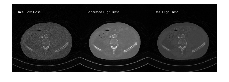
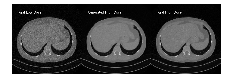
Define the number of test images to use for calculating quality metrics. Randomly select test images to display.

numImagesToDisplay = 3;
idxImagesToDisplay = randi(numel(filesTestHD),1,numImagesToDisplay);

for idx = idxImagesToDisplay
    dsTestHD = partition(timdsTestHD,Files=idx);
    imageHD = read(dsTestHD);
    imageHD = imageHD{1};

    dsTestLD = partition(timdsTestLD,Files=idx);
    imageLD = read(dsTestLD);
    imageLD = imageLD{1};

    imageLD = dlarray(imageLD,"SSCB");
    if canUseGPU
        imageLD = gpuArray(imageLD);
    end

    % Generate high-dose image from low-dose image
    imageHDGenerated = predict(genLD2HD,imageLD);
    imageHDGenerated = gather(extractdata(imageHDGenerated));

    imageLD = gather(extractdata(imageLD));

    imageResultsLDReal = insertText(rescale(imageLD),[40 40],"Real Low Dose", ...
        FontSize=24,TextColor="white",BoxOpacity=0);
    imageResultsHDGen = insertText(rescale(imageHDGenerated),[40 40],"Generated High Dose", ...
        FontSize=24,TextColor="white",BoxOpacity=0);
    imageResultsHDReal = insertText(rescale(imageHD),[40 40],"Real High Dose", ...
        FontSize=24,TextColor="white",BoxOpacity=0);

    figure
    montage({imageResultsLDReal,imageResultsHDGen,imageResultsHDReal},Size=[1 3]);
end

Evaluate Metrics

Initialize variables to store the PSNR and MS-SSIM measurements.

numTest = numel(filesTestLD);
psnrOriginalLD = zeros(numTest,1);
psnrGeneratedHD = zeros(numTest,1);
ssimOriginalLD = zeros(numTest,1);
ssimGeneratedHD = zeros(numTest,1);

Read each pair of test images in the low-dose and high-dose test sets. Generate a high-dose image from the real low-dose image. Then, calculate the PSNR and MS-SSIM of the real low-dose images and the generated high-dose images using the real high-dose image as the ground truth.

reset(timdsTestLD)
reset(timdsTestHD)
for idx = 1:numTest

    imageLD = read(timdsTestLD);
    imageLD = imageLD{1};
    imageHD = read(timdsTestHD);
    imageHD = imageHD{1};

    imageLD = dlarray(imageLD,"SSCB");
    imageHD = dlarray(imageHD,"SSCB");

    if canUseGPU
        imageLD = gpuArray(imageLD);
        imageHD = gpuArray(imageHD);
    end

    % Generate high-dose image from low-dose image
    imageHDGenerated = predict(genLD2HD,imageLD);
    imageHDGenerated = double(imageHDGenerated);
    
    psnrOriginalLD(idx) = psnr(rescale(imageLD),rescale(imageHD));
    psnrGeneratedHD(idx) = psnr(rescale(imageHDGenerated),rescale(imageHD));
    
    ssimOriginalLD(idx) = multissim(rescale(imageLD),rescale(imageHD));
    ssimGeneratedHD(idx) = multissim(rescale(imageHDGenerated),rescale(imageHD));    

end

Calculate and display the mean PNSR and MS-SSIM over the entire test data set. The generated high-dose images have a higher PSNR and MS-SSIM than the original low-dose images.

disp("Average PSNR of original low-dose images: "+mean(psnrOriginalLD));

Average PSNR of original low-dose images: 28.1872

disp("Average PSNR of generated high-dose images: "+mean(psnrGeneratedHD));

Average PSNR of generated high-dose images: 31.1364

disp("Average MS-SSIM of original low-dose images: "+mean(ssimOriginalLD));

Average MS-SSIM of original low-dose images: 0.94467

disp("Average MS-SSIM of generated high-dose images: "+mean(ssimGeneratedHD));

Average MS-SSIM of generated high-dose images: 0.97024

Supporting Functions

Model Gradients Function

The modelGradients function takes as input the two generator and discriminator dlnetwork objects and a mini-batch of input data. The function returns the gradients of the loss with respect to the learnable parameters in the networks and the scores of the four networks. Because the discriminator outputs are not in the range [0, 1], the modelGradients function applies the sigmoid function to convert discriminator outputs into probability scores.

function [genHD2LDGrad,genLD2HDGrad,discLDGrad,discHDGrad, ...
    genHD2LDState,genLD2HDState,scores,metrics, ...
    imagesOutLDAndHDGenerated,imagesOutHDAndLDGenerated] = ...
    modelGradients(genLD2HD,genHD2LD,discLD,discHD,imageHD,imageLD,lambda)

    % Translate images from one domain to another: low-dose to high-dose and
    % vice versa
    [imageLDGenerated,genHD2LDState] = forward(genHD2LD,imageHD);
    [imageHDGenerated,genLD2HDState] = forward(genLD2HD,imageLD);
    
    % Calculate predictions for real images in each domain by the corresponding
    % discriminator networks
    predRealLD = forward(discLD,imageLD);
    predRealHD = forward(discHD,imageHD);
    
    % Calculate predictions for generated images in each domain by the
    % corresponding discriminator networks
    predGeneratedLD = forward(discLD,imageLDGenerated);
    predGeneratedHD = forward(discHD,imageHDGenerated);
    
    % Calculate discriminator losses for real images
    discLDLossReal = lossReal(predRealLD);
    discHDLossReal = lossReal(predRealHD);
    
    % Calculate discriminator losses for generated images
    discLDLossGenerated = lossGenerated(predGeneratedLD);
    discHDLossGenerated = lossGenerated(predGeneratedHD);
    
    % Calculate total discriminator loss for each discriminator network
    discLDLossTotal = 0.5*(discLDLossReal + discLDLossGenerated);
    discHDLossTotal = 0.5*(discHDLossReal + discHDLossGenerated);
    
    % Calculate generator loss for generated images
    genLossHD2LD = lossReal(predGeneratedLD);
    genLossLD2HD = lossReal(predGeneratedHD);
    
    % Complete the round-trip (cycle consistency) outputs by applying the
    % generator to each generated image to get the images in the corresponding
    % original domains
    cycleImageLD2HD2LD = forward(genHD2LD,imageHDGenerated);
    cycleImageHD2LD2HD = forward(genLD2HD,imageLDGenerated);
    
    % Calculate cycle consistency loss between real and generated images
    cycleLossLD2HD2LD = cycleConsistencyLoss(imageLD,cycleImageLD2HD2LD,lambda);
    cycleLossHD2LD2HD = cycleConsistencyLoss(imageHD,cycleImageHD2LD2HD,lambda);
    
    % Calculate identity outputs
    identityImageLD = forward(genHD2LD,imageLD);
    identityImageHD = forward(genLD2HD,imageHD);
     
    % Calculate fidelity loss (SSIM) between the identity outputs
    fidelityLossLD = mean(1-multissim(identityImageLD,imageLD),"all");
    fidelityLossHD = mean(1-multissim(identityImageHD,imageHD),"all");
    
    % Calculate total generator loss
    genLossTotal = genLossHD2LD + cycleLossHD2LD2HD + ...
        genLossLD2HD + cycleLossLD2HD2LD + fidelityLossLD + fidelityLossHD;
    
    % Calculate scores of generators
    genHD2LDScore = mean(sigmoid(predGeneratedLD),"all");
    genLD2HDScore = mean(sigmoid(predGeneratedHD),"all");
    
    % Calculate scores of discriminators
    discLDScore = 0.5*mean(sigmoid(predRealLD),"all") + ...
        0.5*mean(1-sigmoid(predGeneratedLD),"all");
    discHDScore = 0.5*mean(sigmoid(predRealHD),"all") + ...
        0.5*mean(1-sigmoid(predGeneratedHD),"all");
    
    % Combine scores into cell array
    scores = {genHD2LDScore,genLD2HDScore,discLDScore,discHDScore};
    
    % Calculate gradients of generators
    genLD2HDGrad = dlgradient(genLossTotal,genLD2HD.Learnables,RetainData=true);
    genHD2LDGrad = dlgradient(genLossTotal,genHD2LD.Learnables,RetainData=true);
    
    % Calculate gradients of discriminators
    discLDGrad = dlgradient(discLDLossTotal,discLD.Learnables,RetainData=true);
    discHDGrad = dlgradient(discHDLossTotal,discHD.Learnables);

    % Metrics
    psnrLowDose = double(gather(extractdata(mean(psnr(imageLDGenerated,imageLD)))));
    psnrHighDose = double(gather(extractdata(mean(psnr(imageHDGenerated,imageHD)))));
    ssimLowDose = double(gather(extractdata(mean(multissim(imageLDGenerated,imageLD)))));
    ssimHighDose = double(gather(extractdata(mean(multissim(imageHDGenerated,imageHD)))));
    metrics = {psnrLowDose,psnrHighDose,ssimLowDose,ssimHighDose};
    
    % Return mini-batch of images transforming low-dose CT into high-dose CT
    imagesOutLDAndHDGenerated = {imageLD,imageHDGenerated};
    
    % Return mini-batch of images transforming high-dose CT into low-dose CT
    imagesOutHDAndLDGenerated = {imageHD,imageLDGenerated};
end

Loss Functions

Define MSE loss functions for real and generated images.

function loss = lossReal(predictions)
    loss = mean((1-predictions).^2,"all");
end

function loss = lossGenerated(predictions)
    loss = mean((predictions).^2,"all");
end

Define a cycle consistency loss function for real and generated images.

function loss = cycleConsistencyLoss(imageReal,imageGenerated,lambda)
    loss = mean(abs(imageReal-imageGenerated),"all") * lambda;
end

References

[1] Zhu, Jun-Yan, Taesung Park, Phillip Isola, and Alexei A. Efros. “Unpaired Image-to-Image Translation Using Cycle-Consistent Adversarial Networks.” In 2017 IEEE International Conference on Computer Vision (ICCV), 2242–51. Venice: IEEE, 2017. https://doi.org/10.1109/ICCV.2017.244.

[2] McCollough, Cynthia H., Adam C. Bartley, Rickey E. Carter, Baiyu Chen, Tammy A. Drees, Phillip Edwards, David R. Holmes, et al. "Low-dose CT for the detection and classification of metastatic liver lesions: results of the 2016 low dose CT grand challenge." Medical physics 44.10 (2017): e339-e352.

[3] Grants EB017095 and EB017185 (Cynthia McCollough, PI) from the National Institute of Biomedical Imaging and Bioengineering.

[4] AAPM. Low Dose CT Grand Challenge. 2016 Aug; [Online] Available online: https://www.aapm.org/GrandChallenge/LowDoseCT/.

[5] You, Chenyu, Qingsong Yang, Hongming Shan, Lars Gjesteby, Guang Li, Shenghong Ju, Zhuiyang Zhang, et al. “Structurally-Sensitive Multi-Scale Deep Neural Network for Low-Dose CT Denoising.” IEEE Access 6 (2018): 41839–55. https://doi.org/10.1109/ACCESS.2018.2858196.

Acknowledgements

Thanks to Dr. Cynthia McCollough, the Mayo Clinic, the American Association of Physicists in Medicine (AAPM), and grant EB017095 and EB017185 from the National Institute of Biomedical Imaging and Bioengineering for providing the Low-Dose CT Grand Challenge data set.

Related Examples

Unsupervised Medical Image Denoising Using UNIT

More About

Get Started with GANs for Image-to-Image Translation
Datastores for Deep Learning (Deep Learning Toolbox)
Define Custom Training Loops, Loss Functions, and Networks (Deep Learning Toolbox)
Define Model Loss Function for Custom Training Loop (Deep Learning Toolbox)
Specify Training Options in Custom Training Loop (Deep Learning Toolbox)
Train Network Using Custom Training Loop (Deep Learning Toolbox)